Visual Predictive Check (VPC)
Pumas allows you to generate VPC quantiles for your data and model simulations and utilize the Julia plotting capabilities to generate the relevant VPC plots. This is allowed with the vpc function discussed below that returns a VPC object, this can then be passed to the vpc_plot function to generate the plots.
VPC with Simulation
vpc(fpm::AbstractFittedPumasModel;
  samples::Integer = 499
  qreg_method = IP(),
  observations::Vector{Symbol} = [keys(fpm.data[1].observations)[1]],
  stratify_by::Vector{Symbol} = Symbol[],
  quantiles::NTuple{3,Float64}=(0.1, 0.5, 0.9),
  level::Real=0.95,
  ensemblealg=EnsembleSerial(),
  bandwidth=nothing,
  maxnumstrats=[6 for i in 1:length(stratify_by)],
  covariates::Vector{Symbol} = [:time],
  smooth::Bool = true,
  rng::AbstractRNG=default_rng(),
  nodes::Dict = Dict{Tuple{},Vector{Float64}}(),
  nnodes::Integer,
  prediction_correction = false)
Computes the quantiles for VPC for a FittedPumasModel or FittedPumasEMModel with simulated confidence intervals around the empirical quantiles based on samples simulated populations. The following keyword arguments are supported:
samples: The number of simulated populations to generate, defaults to499quantiles::NTuple{3,Float64}: A three-tuple of the quantiles for which the quantiles will be computed. The default is(0.1, 0.5, 0.9)which computes the 10th, 50th and 90th percentile.level::Real: Probability level to use for the simulated confidence intervals. The default is0.95.observations::Vector{Symbol}: The name of the dependent variable to use for the VPCs. The default is the first dependent variable in thePopulation.stratify_by: The covariates to be used for stratification. Takes anVectorof theSymbols of the stratification covariates.ensemblealg: This is passed to thesimobscall for thesamplessimulations. For more description check the docs forsimobs.bandwidth: The kernel bandwidth in the quantile regression. If you are seeingNaNs or an error, increasing the bandwidth should help in most cases. With higher values of thebandwidthyou will get more smoothened plots of the quantiles so it's a good idea to check with your data to pick the rightbandwidth. For a DiscreteVPC, the default value is nothing to indicate automatic bandwidth tuning. For a CensoredVPC, the bandwidth should be given as a tuple where the first value applies to the ContinuousVPC and the second to the DiscreteVPC for the censoring variable. For example,(4.0, nothing)applies a bandwidth of4.0to the ContinuousVPC and automatically tunes the DiscreteVPC. Automatic tuning is only applicable to DiscreteVPCs at this moment.maxnumstrats: The maximum number of strata for each covariate. Takes an Vector with the number of strata for the corresponding covariate, passed instratify_by. It defaults to6for each of the covariates.covariates: The independent variable for VPC, defaults to[:time].smooth: In case of discrete VPC used to determine whether to interpolate the dependent variable if independent variable is continuous, defaults totrue.rng: A random number generator, uses thedefault_rngfromRandomas default.nodes: A Dict of covariate values to use for the local regression.nodes: An integer specifying the number of points to use for the local regressions for each stratum.qreg_method: Defaults toIP(). For most users the method used in quantile regression is not going to be of concern, but if you see large run times switchingqreg_methodtoIP(true)should help in improving the performance with a tradeoff in the accuracy of the fitting.prediction_correction: Default tofalse. Set totrueto enable prediction correction that multiplies all observations with the ratio between the mean prediction and each individuals population prediction.
Hence a vpc call with 100 repetitions of simulation would be:
res = fit(model, data, param, FOCE())
vpc_fpm = vpc(res, samples = 100)
Stratified resampling of the populations for the bootstrap fits based on the wt covariate is performed as follows:
vpc_fpm_stratwt = vpc(res, stratify_by=[:wt])
# run only 100 simulations
vpc_fpm_stratispm = vpc(res, samples = 100, stratify_by=[:isPM])
Prediction correction can be turned on by specifying prediction_correction=true
vpc_fpm = vpc(res, samples = 100, prediction_correction = true)The VPC object obtained as the result contains the following fields:
simulated_quantiles::DataFrame:DataFrameof the simulated quantiles result.popvpc::PopVPC: APopVPCobject with the observation quantiles (data_quantiles), data (data), stratification covariate if specified (stratify_by) and the dependent variable (dv).level::Float64: The simulation CI'slevel.
Since the quantiles are stored as DataFrames it is very easy to use the result of vpc and also export it using CSV.jl to your disk.
vpc_fpm.simulated_quantiles
vpc_fpm.popvpc.data_quantiles

using CSV
CSV.write("sim_quantiles.csv", vpc_fpm.simulated_quantiles)
In Pumas, for models with continuous derived variables (including prediction corrected VPCs), the non-parametric quantile regression approach discussed in Jamsen et al. is used. Discrete and Time to Event models are also supported through the vpc function and can be used without any change in syntax.
Full examples:
Let's take a look at a complete example, first we define the model and generate round-trip data.
julia> model = @model begin @param begin tvcl ∈ RealDomain(lower=0) tvv ∈ RealDomain(lower=0) pmoncl ∈ RealDomain(lower = -0.99) Ω ∈ PDiagDomain(2) σ_prop ∈ RealDomain(lower=0) end @random begin η ~ MvNormal(Ω) end @covariates wt isPM @pre begin CL = tvcl * (1 + pmoncl*isPM) * (wt/70)^0.75 * exp(η[1]) Vc = tvv * (wt/70) * exp(η[2]) end @dynamics Central1 @derived begin cp = @. 1000*(Central / Vc) dv ~ @. Normal(cp, sqrt(cp^2*σ_prop)) end endPumasModel Parameters: tvcl, tvv, pmoncl, Ω, σ_prop Random effects: η Covariates: wt, isPM Dynamical variables: Central Derived: cp, dv Observed: cp, dvjulia> ev = DosageRegimen(100, time=0, addl=2, ii=24)DosageRegimen Row │ time cmt amt evid ii addl rate duration ss route │ Float64 Int64 Float64 Int8 Float64 Int64 Float64 Float64 Int8 NCA.Route ─────┼─────────────────────────────────────────────────────────────────────────────────── 1 │ 0.0 1 100.0 1 24.0 2 0.0 0.0 0 NullRoutejulia> s1 = Subject(id=1, events=ev, covariates=(isPM=1, wt=70))Subject ID: 1 Events: 3 Covariates: isPM, wtjulia> param = ( tvcl = 4.0, tvv = 70, pmoncl = -0.7, Ω = Diagonal([0.09,0.09]), σ_prop = 0.04 )(tvcl = 4.0, tvv = 70, pmoncl = -0.7, Ω = [0.09 0.0; 0.0 0.09], σ_prop = 0.04,)julia> choose_covariates() = (isPM = rand([1, 0]), wt = rand(55:80))choose_covariates (generic function with 1 method)julia> pop_with_covariates = Population(map(i -> Subject(id=i, events=ev, covariates=choose_covariates()),1:10))Population Subjects: 10 Covariates: isPM, wt Observations:julia> obs = simobs(model, pop_with_covariates, param, obstimes=0:1:60)Simulated population (Vector{<:Subject}) Simulated subjects: 10 Simulated variables: cp, dvjulia> simdf = DataFrame(obs)640×15 DataFrame Row │ id time cp dv evid amt cmt rate isPM wt η_1 η_2 ⋯ │ String? Float64 Float64? Float64? Int8? Float64? Symbol? Float64? Int64? Int64? Float64? Floa ⋯ ─────┼────────────────────────────────────────────────────────────────────────────────────────────────────────────────── 1 │ 1 0.0 missing missing 1 100.0 Central 0.0 1 75 0.148927 -0.2 ⋯ 2 │ 1 0.0 1722.83 1660.82 0 missing missing 0.0 1 75 0.148927 -0.2 3 │ 1 1.0 1679.84 1796.04 0 missing missing 0.0 1 75 0.148927 -0.2 4 │ 1 2.0 1637.93 1393.88 0 missing missing 0.0 1 75 0.148927 -0.2 5 │ 1 3.0 1597.06 1687.44 0 missing missing 0.0 1 75 0.148927 -0.2 ⋯ 6 │ 1 4.0 1557.21 1353.73 0 missing missing 0.0 1 75 0.148927 -0.2 7 │ 1 5.0 1518.35 1123.05 0 missing missing 0.0 1 75 0.148927 -0.2 8 │ 1 6.0 1480.47 1186.22 0 missing missing 0.0 1 75 0.148927 -0.2 9 │ 1 7.0 1443.53 785.65 0 missing missing 0.0 1 75 0.148927 -0.2 ⋯ 10 │ 1 8.0 1407.51 1860.71 0 missing missing 0.0 1 75 0.148927 -0.2 11 │ 1 9.0 1372.39 956.926 0 missing missing 0.0 1 75 0.148927 -0.2 ⋮ │ ⋮ ⋮ ⋮ ⋮ ⋮ ⋮ ⋮ ⋮ ⋮ ⋮ ⋮ ⋱ 631 │ 10 51.0 1964.28 1703.23 0 missing missing 0.0 0 66 -0.32187 0.0 632 │ 10 52.0 1886.56 1942.05 0 missing missing 0.0 0 66 -0.32187 0.0 ⋯ 633 │ 10 53.0 1811.92 1141.5 0 missing missing 0.0 0 66 -0.32187 0.0 634 │ 10 54.0 1740.23 1510.94 0 missing missing 0.0 0 66 -0.32187 0.0 635 │ 10 55.0 1671.38 1959.94 0 missing missing 0.0 0 66 -0.32187 0.0 636 │ 10 56.0 1605.25 1335.0 0 missing missing 0.0 0 66 -0.32187 0.0 ⋯ 637 │ 10 57.0 1541.73 1946.85 0 missing missing 0.0 0 66 -0.32187 0.0 638 │ 10 58.0 1480.73 1924.21 0 missing missing 0.0 0 66 -0.32187 0.0 639 │ 10 59.0 1422.15 1415.06 0 missing missing 0.0 0 66 -0.32187 0.0 640 │ 10 60.0 1365.88 1459.32 0 missing missing 0.0 0 66 -0.32187 0.0 ⋯ 4 columns and 619 rows omittedjulia> data = read_pumas(simdf, time=:time, covariates=[:isPM, :wt])Population Subjects: 10 Covariates: isPM, wt Observations: dvjulia> res = fit(model, data, param, Pumas.FOCE())[ Info: Checking the initial parameter values. [ Info: The initial negative log likelihood and its gradient are finite. Check passed. Iter Function value Gradient norm 0 4.210123e+03 1.427956e+01 * time: 0.025641918182373047 1 4.208916e+03 1.120037e+01 * time: 1.4024410247802734 2 4.208633e+03 3.290248e+00 * time: 1.4119019508361816 3 4.208263e+03 1.607001e+00 * time: 1.4179730415344238 4 4.208167e+03 2.140971e+00 * time: 1.4279439449310303 5 4.207993e+03 3.232515e+00 * time: 1.4348669052124023 6 4.207883e+03 7.334774e-01 * time: 1.4416818618774414 7 4.207878e+03 8.057361e-02 * time: 1.4483439922332764 8 4.207878e+03 5.206846e-02 * time: 1.454577922821045 9 4.207878e+03 6.027372e-03 * time: 1.4607658386230469 10 4.207878e+03 3.995105e-03 * time: 1.4665088653564453 11 4.207878e+03 1.089705e-03 * time: 1.4724030494689941 12 4.207878e+03 1.089705e-03 * time: 1.4835140705108643 13 4.207878e+03 9.898004e-04 * time: 1.4900188446044922 FittedPumasModel Successful minimization: true Likelihood approximation: FOCE Log-likelihood value: -4207.8776 Number of subjects: 10 Number of parameters: Fixed Optimized 0 6 Observation records: Active Missing dv: 610 0 Total: 610 0 --------------------- Estimate --------------------- tvcl 3.581 tvv 75.187 pmoncl -0.73905 Ω₁,₁ 0.085148 Ω₂,₂ 0.048751 σ_prop 0.041515 ---------------------
julia> vpc_fpm = vpc(res);

julia> vpc_plot(vpc_fpm)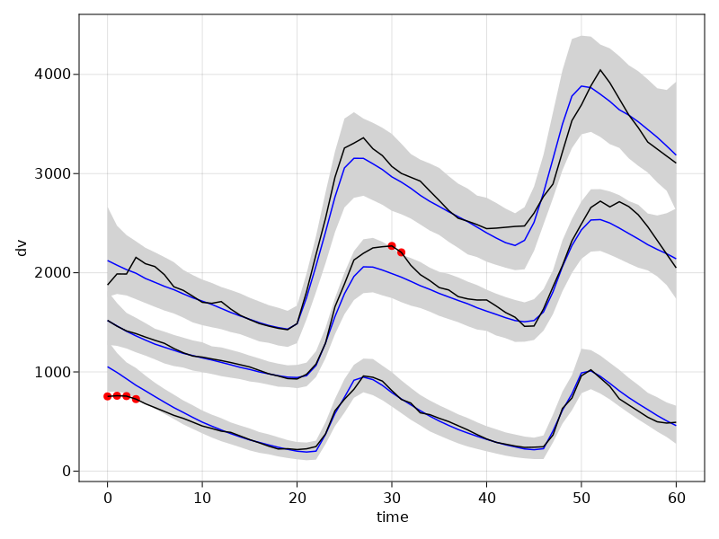
Alternatively, using a PumasEMModel
emmodel = @emmodel begin
  @random begin
    CLdw ~ 1 + isPM | LogNormal # CLdw = μ_CL * exp(μ_CL_isPM * isPM) * exp(η_CL)
    Vcdw ~ 1        | LogNormal # Vcdw = μ_Vc * exp(η_Vc)
  end
  @covariates wt
  @pre begin
    CL = CLdw * (wt/70)^0.75
    Vc = Vcdw * (wt/70)
  end
  @dynamics Central1
  @post begin
    cp = 1000 * Central / Vc
  end
  @error begin
    dv ~ ProportionalNormal(cp)
  end
end

emparam = (
    CLdw = (4.0, -1.2), # -1.2 ≈ log(1 - 0.7) = log(1 - pmoncl)
    Vcdw    = 70,
    Ω = (0.09,0.09),
    σ = (0.04,)
)

emres = fit(emmodel, data, emparam, Pumas.LaplaceI())

vpc_emfpm = vpc(emres)
Note that because isPM equals either 0 or 1, pmoncl = exp(μ_CL_isPM) - 1, allowing us to perform a change of variables and express the earlier PumasModel as a PumasEMModel.
In PumasModels and PumasEMModels, you can increase performance by preprocessing covariates. Instead of wt, you can try storing (wt/70) and (wt/70)^0.75 as appropriately named covariates.
vpc_plot(vpc_emfpm)
Let's generate a VPC stratified on isPM covariate with stratify_by. Note that multiple covariates can be passed to stratify_by to get cross stratified VPC plots, in that case the maxnumstrats will have to be adjusted accordingly.
resem_saem = fit(emmodel, data, (CLdw = (5.0,0.0), Vcdw = 50.0), Pumas.SAEM())

vpc_fpmem_saem = vpc(resem_saem, samples = 100)
vpc_plot(vpc_fpmem_saem)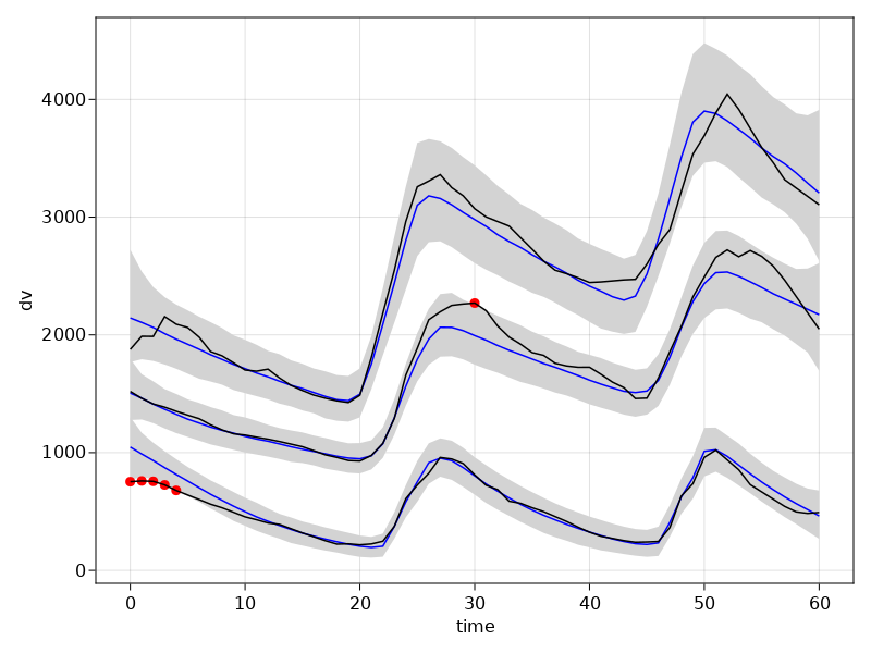
When fitting with SAEM, it is strongly recommended to use values for the Ω parameters much larger than your estimates of the true values, or to avoid providing them so they default to 1.0 along the diagonal. Using small values such as emparams will result in convergence failure.
vpc_fpm = vpc(res, stratify_by = [:isPM])
vpc_plot(vpc_fpm)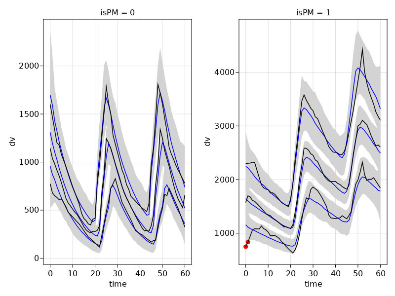
vpc_saem_fpm = vpc(resem_saem, stratify_by = [:isPM]);
vpc_plot(vpc_saem_fpm)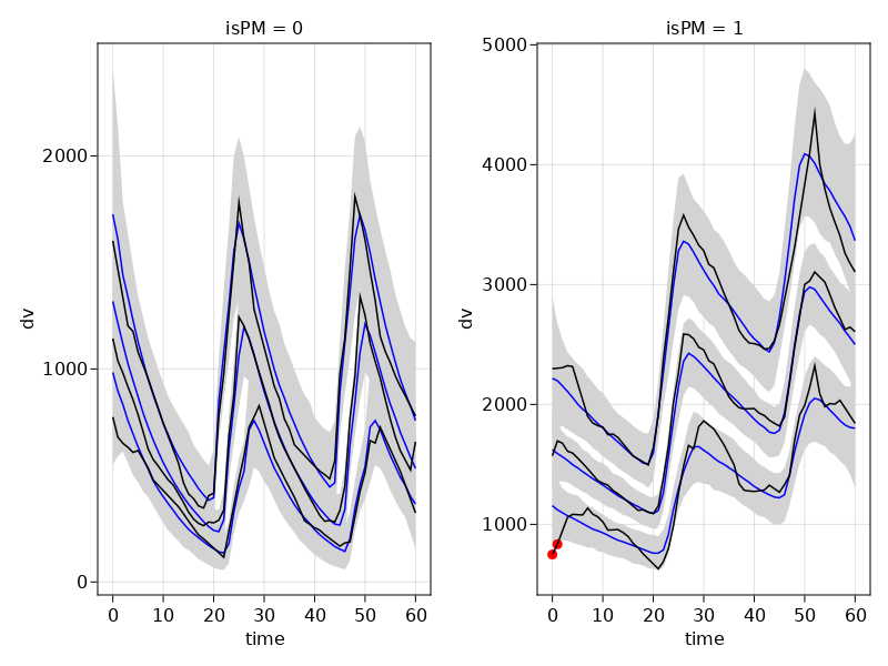
Let's pass in the time grid with the obstimes keyword argument to vpc for the simulation time points.
vpc_fpm = vpc(res, 100, obstimes = 0.0:5:60.0)
vpc_plot(vpc_fpm)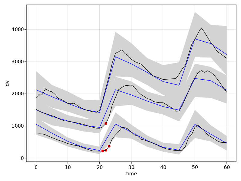
By specifying the plot and the path the VPC plot can be saved to the disk as below:
p = vpc_plot(vpc_fpm)
CairoMakie.save("obstimesvpc.png", p)
More examples of VPC plots can be found in the plotting page's vpc_plot section.
If your vpc run gives you an error message similar to ERROR: LinearAlgebra.LAPACKException(2), increasing the bandwidth should fix it in most cases.
For most users, the method used in quantile regression is not going to be of concern, but if you see large run times switching qreg_method to IP(true) after loading QuantileRegressions.jl should help in improving the performance with a tradeoff in the accuracy of the regression fitting.
Prediction corrected VPCs (pcVPCs) are work in progress and will become available soon.
VPC after Simulation
vpc(sims;
  qreg_method=IP(),
  observations::Array{Symbol}, # defaults to all observations
  stratify_by::Array{Symbol} = Symbol[],
  quantiles::NTuple{3,Float64} = (0.1, 0.5, 0.9),
  level::Real = 0.95,
  ensemblealg = EnsembleSerial(),
  bandwidth::Real = 2,
  maxnumstrats::Array{<:Integer} = [6 for i in 1:length(stratify_by)],
  covariates::Array{Symbol} = [:time],
  smooth::Bool = true,
)
It is also possible to run the VPC as a post-processing step on arbitrary simulation output sims from any simobs function call. For more on simulations and how to use simobs, check the Simulation of Pumas Models section of the documentation.
Example:
The following is an example of simulating from a bootstrap result and then plotting a VPC using the simulations.
julia> model = @model begin @param begin tvcl ∈ RealDomain(lower=0) tvv ∈ RealDomain(lower=0) pmoncl ∈ RealDomain(lower = -0.99) Ω ∈ PDiagDomain(2) σ_prop ∈ RealDomain(lower=0) end @random begin η ~ MvNormal(Ω) end @covariates wt isPM @pre begin CL = tvcl * (1 + pmoncl*isPM) * (wt/70)^0.75 * exp(η[1]) Vc = tvv * (wt/70) * exp(η[2]) end @dynamics Central1 @derived begin cp = @. 1000*(Central / Vc) dv ~ @. Normal(cp, sqrt(cp^2*σ_prop)) end endPumasModel Parameters: tvcl, tvv, pmoncl, Ω, σ_prop Random effects: η Covariates: wt, isPM Dynamical variables: Central Derived: cp, dv Observed: cp, dvjulia> ev = DosageRegimen(100, time=0, addl=2, ii=24)DosageRegimen Row │ time cmt amt evid ii addl rate duration ss route │ Float64 Int64 Float64 Int8 Float64 Int64 Float64 Float64 Int8 NCA.Route ─────┼─────────────────────────────────────────────────────────────────────────────────── 1 │ 0.0 1 100.0 1 24.0 2 0.0 0.0 0 NullRoutejulia> s1 = Subject(id=1, events=ev, covariates=(isPM=1, wt=70))Subject ID: 1 Events: 3 Covariates: isPM, wtjulia> param = ( tvcl = 4.0, tvv = 70, pmoncl = -0.7, Ω = Diagonal([0.09,0.09]), σ_prop = 0.04 )(tvcl = 4.0, tvv = 70, pmoncl = -0.7, Ω = [0.09 0.0; 0.0 0.09], σ_prop = 0.04,)julia> choose_covariates() = (isPM = rand([1, 0]), wt = rand(55:80))choose_covariates (generic function with 1 method)julia> pop_with_covariates = Population(map(i -> Subject(id=i, events=ev, covariates=choose_covariates()),1:10))Population Subjects: 10 Covariates: isPM, wt Observations:julia> obs = simobs(model, pop_with_covariates, param, obstimes=0:1:60)Simulated population (Vector{<:Subject}) Simulated subjects: 10 Simulated variables: cp, dvjulia> simdf = DataFrame(obs)640×15 DataFrame Row │ id time cp dv evid amt cmt rate isPM wt η_1 η_2 ⋯ │ String? Float64 Float64? Float64? Int8? Float64? Symbol? Float64? Int64? Int64? Float64? Floa ⋯ ─────┼────────────────────────────────────────────────────────────────────────────────────────────────────────────────── 1 │ 1 0.0 missing missing 1 100.0 Central 0.0 1 59 -0.203496 -0.3 ⋯ 2 │ 1 0.0 2349.06 2834.12 0 missing missing 0.0 1 59 -0.203496 -0.3 3 │ 1 1.0 2302.01 2088.25 0 missing missing 0.0 1 59 -0.203496 -0.3 4 │ 1 2.0 2255.91 2433.17 0 missing missing 0.0 1 59 -0.203496 -0.3 5 │ 1 3.0 2210.73 2843.99 0 missing missing 0.0 1 59 -0.203496 -0.3 ⋯ 6 │ 1 4.0 2166.45 2695.38 0 missing missing 0.0 1 59 -0.203496 -0.3 7 │ 1 5.0 2123.07 2218.7 0 missing missing 0.0 1 59 -0.203496 -0.3 8 │ 1 6.0 2080.55 2576.84 0 missing missing 0.0 1 59 -0.203496 -0.3 9 │ 1 7.0 2038.88 1923.04 0 missing missing 0.0 1 59 -0.203496 -0.3 ⋯ 10 │ 1 8.0 1998.04 1779.28 0 missing missing 0.0 1 59 -0.203496 -0.3 11 │ 1 9.0 1958.03 2281.98 0 missing missing 0.0 1 59 -0.203496 -0.3 ⋮ │ ⋮ ⋮ ⋮ ⋮ ⋮ ⋮ ⋮ ⋮ ⋮ ⋮ ⋮ ⋱ 631 │ 10 51.0 1818.44 1934.81 0 missing missing 0.0 1 71 0.11475 0.5 632 │ 10 52.0 1798.92 1829.57 0 missing missing 0.0 1 71 0.11475 0.5 ⋯ 633 │ 10 53.0 1779.61 2487.2 0 missing missing 0.0 1 71 0.11475 0.5 634 │ 10 54.0 1760.5 1907.77 0 missing missing 0.0 1 71 0.11475 0.5 635 │ 10 55.0 1741.61 1150.23 0 missing missing 0.0 1 71 0.11475 0.5 636 │ 10 56.0 1722.91 1945.88 0 missing missing 0.0 1 71 0.11475 0.5 ⋯ 637 │ 10 57.0 1704.42 1757.16 0 missing missing 0.0 1 71 0.11475 0.5 638 │ 10 58.0 1686.12 815.761 0 missing missing 0.0 1 71 0.11475 0.5 639 │ 10 59.0 1668.03 1314.08 0 missing missing 0.0 1 71 0.11475 0.5 640 │ 10 60.0 1650.12 2227.83 0 missing missing 0.0 1 71 0.11475 0.5 ⋯ 4 columns and 619 rows omittedjulia> data = read_pumas(simdf, time=:time, covariates=[:isPM, :wt])Population Subjects: 10 Covariates: isPM, wt Observations: dvjulia> res = fit(model, data, param, Pumas.FOCE())[ Info: Checking the initial parameter values. [ Info: The initial negative log likelihood and its gradient are finite. Check passed. Iter Function value Gradient norm 0 4.291898e+03 8.459415e+00 * time: 6.914138793945312e-5 1 4.291565e+03 3.821093e+00 * time: 0.06625699996948242 2 4.291305e+03 3.199247e+00 * time: 0.07520914077758789 3 4.290736e+03 2.441670e+00 * time: 0.08396005630493164 4 4.290554e+03 3.162458e+00 * time: 0.0925600528717041 5 4.289690e+03 2.555937e+00 * time: 0.10087704658508301 6 4.289621e+03 2.258847e+00 * time: 0.10643315315246582 7 4.289534e+03 7.641300e-01 * time: 0.11186504364013672 8 4.289529e+03 4.090504e-01 * time: 0.11703896522521973 9 4.289528e+03 1.198260e-01 * time: 0.12206006050109863 10 4.289527e+03 2.912963e-02 * time: 0.12705707550048828 11 4.289527e+03 4.122647e-03 * time: 0.13205909729003906 12 4.289527e+03 4.122647e-03 * time: 0.14523792266845703 13 4.289527e+03 4.122647e-03 * time: 0.158066987991333 FittedPumasModel Successful minimization: true Likelihood approximation: FOCE Log-likelihood value: -4289.5274 Number of subjects: 10 Number of parameters: Fixed Optimized 0 6 Observation records: Active Missing dv: 610 0 Total: 610 0 --------------------- Estimate --------------------- tvcl 3.5643 tvv 72.656 pmoncl -0.65651 Ω₁,₁ 0.033152 Ω₂,₂ 0.067815 σ_prop 0.038743 ---------------------julia> inf = infer(res, Pumas.Bootstrap(samples = 100))Progress: 2%|█▋ | ETA: 0:07:14 Progress: 3%|██▍ | ETA: 0:05:03Progress: 4%|███▎ | ETA: 0:03:45Progress: 5%|████ | ETA: 0:03:02 Progress: 6%|████▉ | ETA: 0:02:30 Progress: 7%|█████▋ | ETA: 0:02:17 Progress: 8%|██████▌ | ETA: 0:02:00 Progress: 11%|████████▉ | ETA: 0:01:27 Progress: 18%|██████████████▋ | ETA: 0:00:54 Progress: 25%|████████████████████▎ | ETA: 0:00:39 Progress: 27%|█████████████████████▉ | ETA: 0:00:36 Progress: 28%|██████████████████████▋ | ETA: 0:00:34 Progress: 30%|████████████████████████▎ | ETA: 0:00:32 Progress: 32%|█████████████████████████▉ | ETA: 0:00:29 Progress: 33%|██████████████████████████▊ | ETA: 0:00:28 Progress: 35%|████████████████████████████▍ | ETA: 0:00:26 Progress: 36%|█████████████████████████████▏ | ETA: 0:00:25 Progress: 39%|███████████████████████████████▋ | ETA: 0:00:23Progress: 40%|████████████████████████████████▍ | ETA: 0:00:22 Progress: 41%|█████████████████████████████████▎ | ETA: 0:00:21 Progress: 42%|██████████████████████████████████ | ETA: 0:00:21 Progress: 43%|██████████████████████████████████▉ | ETA: 0:00:20 Progress: 44%|███████████████████████████████████▋ | ETA: 0:00:20 Progress: 49%|███████████████████████████████████████▊ | ETA: 0:00:17 Progress: 51%|█████████████████████████████████████████▎ | ETA: 0:00:16 Progress: 59%|███████████████████████████████████████████████▊ | ETA: 0:00:12 Progress: 64%|███████████████████████████████████████████████████▉ | ETA: 0:00:10 Progress: 69%|███████████████████████████████████████████████████████▉ | ETA: 0:00:09 Progress: 71%|█████████████████████████████████████████████████████████▌ | ETA: 0:00:08 Progress: 73%|███████████████████████████████████████████████████████████▏ | ETA: 0:00:07 Progress: 81%|█████████████████████████████████████████████████████████████████▋ | ETA: 0:00:05 Progress: 82%|██████████████████████████████████████████████████████████████████▍ | ETA: 0:00:05 Progress: 83%|███████████████████████████████████████████████████████████████████▎ | ETA: 0:00:04 Progress: 84%|████████████████████████████████████████████████████████████████████ | ETA: 0:00:04Progress: 85%|████████████████████████████████████████████████████████████████████▉ | ETA: 0:00:04 Progress: 93%|███████████████████████████████████████████████████████████████████████████▍ | ETA: 0:00:02 Progress: 96%|█████████████████████████████████████████████████████████████████████████████▊ | ETA: 0:00:01 Progress: 98%|███████████████████████████████████████████████████████████████████████████████▍ | ETA: 0:00:00 Progress: 100%|█████████████████████████████████████████████████████████████████████████████████| Time: 0:00:23 ┌ Info: Bootstrap inference finished. │ Total resampled fits = 100 │ Success rate = 1.0 └ Unique resampled populations = 100 Bootstrap inference results Successful minimization: true Likelihood approximation: FOCE Log-likelihood value: -4289.5274 Number of subjects: 10 Number of parameters: Fixed Optimized 0 6 Observation records: Active Missing dv: 610 0 Total: 610 0 -------------------------------------------------------------------- Estimate SE 95.0% C.I. -------------------------------------------------------------------- tvcl 3.5643 0.39768 [ 2.9374 ; 4.3896 ] tvv 72.656 6.6339 [62.231 ; 86.846 ] pmoncl -0.65651 0.048474 [-0.74322 ; -0.57146 ] Ω₁,₁ 0.033152 0.011907 [ 1.5179e-8; 0.044716] Ω₂,₂ 0.067815 0.024863 [ 0.020753 ; 0.11463 ] σ_prop 0.038743 0.0022272 [ 0.035269 ; 0.043319] -------------------------------------------------------------------- Successful fits: 100 out of 100 Unique resampled populations: 100 No stratification.julia> sims = simobs(inf, samples = 50)50-element Vector{Vector{Pumas.SimulatedObservations{PumasModel{(tvcl = 1, tvv = 1, pmoncl = 1, Ω = 2, σ_prop = 1), 2, (:Central,), ParamSet{NamedTuple{(:tvcl, :tvv, :pmoncl, :Ω, :σ_prop), Tuple{RealDomain{Int64, TransformVariables.Infinity{true}, Int64}, RealDomain{Int64, TransformVariables.Infinity{true}, Int64}, RealDomain{Float64, TransformVariables.Infinity{true}, Float64}, PDiagDomain{PDMats.PDiagMat{Float64, Vector{Float64}}}, RealDomain{Int64, TransformVariables.Infinity{true}, Int64}}}}, Main.var"#17#24", Pumas.TimeDispatcher{Main.var"#18#25", Main.var"#19#26"}, Nothing, Main.var"#21#28", Central1, Main.var"#22#29", Main.var"#23#30", Nothing}, Subject{NamedTuple{(:dv,), Tuple{Vector{Union{Missing, Float64}}}}, Pumas.ConstantCovar{NamedTuple{(:isPM, :wt), Tuple{Int64, Int64}}}, Vector{Pumas.Event{Float64, Float64, Float64, Float64, Float64, Float64, Symbol}}, Vector{Float64}}, Vector{Float64}, NamedTuple{(:tvcl, :tvv, :pmoncl, :Ω, :σ_prop), Tuple{Float64, Float64, Float64, PDMats.PDiagMat{Float64, Vector{Float64}}, Float64}}, NamedTuple{(:η,), Tuple{Vector{Float64}}}, NamedTuple{(:isPM, :wt), Tuple{Vector{Int64}, Vector{Int64}}}, NamedTuple{(:alg, :callback), Tuple{CompositeAlgorithm{Tuple{Tsit5{typeof(OrdinaryDiffEq.trivial_limiter!), typeof(OrdinaryDiffEq.trivial_limiter!), Static.False}, Rosenbrock23{1, true, LinearSolve.LUFactorization{RowMaximum}, typeof(OrdinaryDiffEq.DEFAULT_PRECS), Val{:forward}, true, nothing}}, AutoSwitch{Tsit5{typeof(OrdinaryDiffEq.trivial_limiter!), typeof(OrdinaryDiffEq.trivial_limiter!), Static.False}, Rosenbrock23{1, true, LinearSolve.LUFactorization{RowMaximum}, typeof(OrdinaryDiffEq.DEFAULT_PRECS), Val{:forward}, true, nothing}, Rational{Int64}, Int64}}, Nothing}}, Pumas.PKPDAnalyticalSolution{StaticArraysCore.SVector{1, Float64}, 2, Vector{StaticArraysCore.SVector{1, Float64}}, Vector{Float64}, Vector{StaticArraysCore.SVector{1, Float64}}, Vector{StaticArraysCore.SVector{1, Float64}}, Pumas.Returns{NamedTuple{(:CL, :Vc), Tuple{Float64, Float64}}}, Pumas.AnalyticalPKPDProblem{StaticArraysCore.SVector{1, Float64}, Float64, false, Central1, Vector{Pumas.Event{Float64, Float64, Float64, Float64, Float64, Float64, Int64}}, Vector{Float64}, Pumas.Returns{NamedTuple{(:CL, :Vc), Tuple{Float64, Float64}}}}}, NamedTuple{(), Tuple{}}, NamedTuple{(:CL, :Vc), Tuple{Vector{Float64}, Vector{Float64}}}, NamedTuple{(:cp, :dv), Tuple{Vector{Float64}, Vector{Float64}}}}}}: Simulated population (Vector{<:Subject}), n = 10, variables: cp, dv Simulated population (Vector{<:Subject}), n = 10, variables: cp, dv Simulated population (Vector{<:Subject}), n = 10, variables: cp, dv Simulated population (Vector{<:Subject}), n = 10, variables: cp, dv Simulated population (Vector{<:Subject}), n = 10, variables: cp, dv Simulated population (Vector{<:Subject}), n = 10, variables: cp, dv Simulated population (Vector{<:Subject}), n = 10, variables: cp, dv Simulated population (Vector{<:Subject}), n = 10, variables: cp, dv Simulated population (Vector{<:Subject}), n = 10, variables: cp, dv Simulated population (Vector{<:Subject}), n = 10, variables: cp, dv Simulated population (Vector{<:Subject}), n = 10, variables: cp, dv Simulated population (Vector{<:Subject}), n = 10, variables: cp, dv Simulated population (Vector{<:Subject}), n = 10, variables: cp, dv ⋮ Simulated population (Vector{<:Subject}), n = 10, variables: cp, dv Simulated population (Vector{<:Subject}), n = 10, variables: cp, dv Simulated population (Vector{<:Subject}), n = 10, variables: cp, dv Simulated population (Vector{<:Subject}), n = 10, variables: cp, dv Simulated population (Vector{<:Subject}), n = 10, variables: cp, dv Simulated population (Vector{<:Subject}), n = 10, variables: cp, dv Simulated population (Vector{<:Subject}), n = 10, variables: cp, dv Simulated population (Vector{<:Subject}), n = 10, variables: cp, dv Simulated population (Vector{<:Subject}), n = 10, variables: cp, dv Simulated population (Vector{<:Subject}), n = 10, variables: cp, dv Simulated population (Vector{<:Subject}), n = 10, variables: cp, dv Simulated population (Vector{<:Subject}), n = 10, variables: cp, dvjulia> vpc_sims = vpc(sims);[ Info: Detected 50 scenarios and 10 subjects in the input simulations. Running VPC. [ Info: Continuous VPC Progress: 4%|███▎ | ETA: 0:01:18 Progress: 10%|████████▏ | ETA: 0:00:30 Progress: 16%|█████████████ | ETA: 0:00:18 Progress: 22%|█████████████████▉ | ETA: 0:00:13 Progress: 28%|██████████████████████▋ | ETA: 0:00:09 Progress: 34%|███████████████████████████▌ | ETA: 0:00:07 Progress: 40%|████████████████████████████████▍ | ETA: 0:00:06 Progress: 46%|█████████████████████████████████████▎ | ETA: 0:00:05 Progress: 52%|██████████████████████████████████████████▏ | ETA: 0:00:04 Progress: 58%|███████████████████████████████████████████████ | ETA: 0:00:03 Progress: 64%|███████████████████████████████████████████████████▉ | ETA: 0:00:03 Progress: 70%|████████████████████████████████████████████████████████▊ | ETA: 0:00:02 Progress: 76%|█████████████████████████████████████████████████████████████▌ | ETA: 0:00:02 Progress: 82%|██████████████████████████████████████████████████████████████████▍ | ETA: 0:00:01 Progress: 88%|███████████████████████████████████████████████████████████████████████▎ | ETA: 0:00:01 Progress: 94%|████████████████████████████████████████████████████████████████████████████▏ | ETA: 0:00:00 Progress: 100%|█████████████████████████████████████████████████████████████████████████████████| Time: 0:00:05julia> vpc_plot(vpc_sims)FigureAxisPlot()