Bayesian Workflow
You can use Pumas to perform a full Bayesian analysis workflow including:
- Complex hierarchical and dynamics-based model definition
- Data wrangling
- Simulation
- Posterior sampling
- Convergence diagnostics
- Posterior predictions and probabilistic queries
- Model selection and plotting
In this section, an overview of the Bayesian workflow in Pumas will be presented. To better understand this section, some familiarity with Bayesian inference is required. You can learn about the basics of Bayesian inference using [3]. It may also be useful to read this section more than once to fully understand all the concepts since some concepts are related to each other in a circular fashion.
Table of contents
- Bayesian Workflow
- Table of contents
- Advantages of Bayesian analysis
- Data wrangling and dose regimens
- Model definition
- Simulating from the prior model
- Sampling from the posterior using MCMC
- Convergence and diagnostics
- Posterior queries
- Cross-validation and model selection
Advantages of Bayesian analysis
The Bayesian workflow allows analysts to:
- Incorporate domain knowledge and insights from previous studies using prior distributions.
- Quantify the epistemic uncertainty in the model parameters' values. Parameter values can be uncertain in reality due to model non-identifiability or practical non-identifiability issues because of lack of data.
This epistemic uncertainty can be further propagated forward via simulation to get a distribution of predictions which when used to make decisions, e.g. dosing decisions, can make those decisions more robust to changes in the parameter values. The above are advantages of Bayesian analysis which the traditional frequentist workflow typically doesn't have a satisfactory answer for. Using bootstrapping or asymptotic estimates of standard errors can be considered somewhat ad-hoc and assumptions methods to quantify uncertainty in the parameter estimates when Bayesian inference uses the established theory of probability to more rigorously quantify said uncertainty with fewer assumptions about the model.
It is important to note that one can still reap the second benefit of Bayesian analysis due to its flexibility even when little to no domain knowledge is imposed on the model. So the Bayesian workflow doesn't force you to incorporate your domain knowledge, but it empowers you to if you want.
Data wrangling and dose regimens
Data wrangling for Bayesian inference in Pumas is identical to regular data wrangling for frequentist workflows. The data can be read from files to data frames and converted to a Pumas population. For more on data wrangling in Pumas and defining dosage regimens, you can check the Dosage Regimens, Subjects, and Populations section of the documentation.
Model definition
You can define a probabilistic hierarchical model using the @model macro in Pumas. The @model macro is extensively explained in the Defining NLME models in Pumas section of the documentation. The Bayesian workflow in Pumas works with the full range of models you can write using the @model macro including models with complicated dynamics, dose regimens and a large number of population or subject-specific parameters.
Prior distributions available
| (-∞, ∞) | (0, ∞) |
|---|---|
 |  |
| (0, ∞) | (0, 1) |
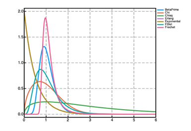 |  |
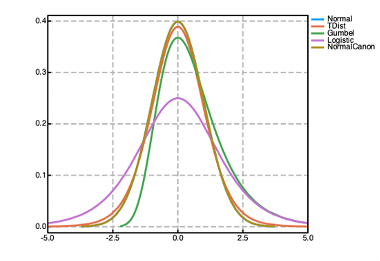
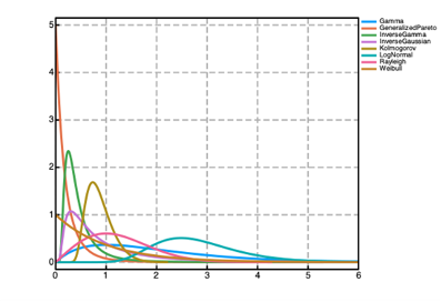
Prior distributions can be used to encode prior knowledge about the values of the parameters in both the @param and @random blocks in a Pumas model. A number of prior distributions are available for use in Pumas with widely different probability density functions (PDFs) as shown in the figure above. Univariate distributions can be used as priors for scalar parameters. Multivariate distributions can be used as priors for vector parameters. And finally matrix-variate distributions can be used as priors for matrix parameters. The following are some of the most used priors available in Pumas (although there are many more available):
Normal(μ, σ): univariate normal distributions with support(-∞, ∞), meanμand standard deviationσ.LogNormal(μ, σ): univariate log normal distribution with support(0, ∞)and a base normal distribution of meanμand standard deviationσ.MvNormal(μ, Σ): multivariate normal distribution with mean vectorμand covariance matrixΣ.Σcan also be a diagonal matrix, e.g.Diagonal([1.0, 1.0]). If a scalar is input forΣ, it is treated as the standard deviation of all the independent random variables. You can also passΣalone as a matrix, e.g.MvNormal(Σ::AbstractMatrix), and the means will be assumed to be 0.MvLogNormal(μ, Σ): a multivariate log normal distribution over positive vectors with a base multivariate normal distribution with parametersμandΣ. TheμandΣhere are identical to theMvNormalones above.Cauchy(μ, σ): a univariate Cauchy distribution with support(-∞, ∞)locationμand scaleσ.Constrained(dist; lower, upper): a constrained prior distribution with a fixed support(lower, upper)and a fixed base distributiondistthat could be any univariate or multivariate distribution.lowerandupperare optional keyword arguments that set the bounds on the random variables' support. Whendistis a univariate distribution,loweranduppershould be scalars. When constraining multivariate distributions,loweranduppercan be vectors or scalars. If scalar, the same bound will be used for all random variables. If unset,lowerwill be-∞andupperwill be∞. There is also atruncateddistribution which is different fromConstrainedin that it allows the base distribution to be a function of the model's parameters buttruncatedonly supports univariate base distributions. In general, it's recommended to useConstrainedin the@paramblock andtruncatedin the@randomand@derivedblocks. Examples:Constrained(Normal(); lower = 0.0)is a half normal distribution.Constrained(Cauchy(); lower = 0.0)is a half Cauchy distribution.Constrained(MvNormal([0.0, 0.0], [1.0 0.0; 0.0 1.0]); lower = 0.0)is a constrained multivariate normal distribution.
truncated(dist; lower, upper): similar toConstrainedwith fixed lower and upper boundslowerandupperrespectively and a base distributiondist. Intruncated, the base distributiondistis allowed to depend on the model's parameters and the renormalization constant is computed in every log PDF evaluation. However, the lower and upper bounds must be fixed constants andtruncatedonly supports univariate base distribution. In general, it's recommended to useConstrainedin the@paramblock andtruncatedin the@randomand@derivedblocks. Examples:truncated(Normal(); lower = 0.0)is a half normal distribution.truncated(Cauchy(); lower = 0.0)is a half Cauchy distribution.truncated(Normal(); upper = 0.0)is a negative half normal distribution.
Uniform(l, u): a univariate uniform distribution with lower and upper boundslandurespectively.LKJ(d, η): a matrix-variate LKJ prior over correlation matrices of sized × d.ηis the positive shape parameter of the LKJ prior.Wishart(ν, S): a matrix-variate Wishart distribution overd × dpositive definite matrices withνdegrees of freedom and a positive definiteSscale matrix.InverseWishart(ν, ψ): a matrix-variate inverse Wishart distribution overd × dpositive definite matrices withνdegrees of freedom and a positive definite scale matrixψ.Beta(α, β): a univariate Beta distribution with support from 0 to 1 and shape parametersαandβ.Gamma(α, θ): a univariate Gamma distribution over positive numbers with shape parameterαand scaleθ.Logistic(μ, θ): a univariate logistic distribution with support(-∞, ∞), locationμand scaleθ.LogitNormal(μ, σ): a univariate logit normal distribution with support(0, 1)and a base normal distribution with meanμand standard deviationσ.TDist(ν): a univariate Student's T distribution with support(-∞, ∞),νdegrees of freedom and mean 0. To change the mean of the T distribution, you can shift its location (shown below).μ + σ * dist: a scaled and translated univariate distribution with a base distributiondist. The base distribution's random variable is first scaled byσand then translated byμ. Example:1 + 2 * TDist(2)is a scaled and translated Student's $t$ distribution. The mean of a scaled and translated distribution isμ + σ × mean(dist)and the standard deviation isσ × std(dist).Laplace(μ, σ): a univariate Laplace distribution with support(-∞, ∞), locationμand scaleθ.Exponential(θ): a univariate exponential distribution with support(0, ∞)and scaleθ.(Improper) flat priors: instead of using a distribution, one can specify a domain instead such as a
VectorDomainfor vector parameters,PSDDomainfor positive definite parameters orCorrDomainfor correlation matrix parameters. Those domains are treated in Pumas a flat prior. If the domain is open, this would be an improper prior. For about domains, see the Defining NLME models in Pumas section in the documentation or type?followed by the domain name in the REPL for help.
More generally, all distributions supported in the @random block can be used as prior distributions.
Example: 2-compartment PK model
The following is an example of a 2-compartment population PK model written in Pumas:
poppk2cpt = @model begin
    @param begin
        tvcl ~ LogNormal(log(10), 0.25)
        tvq ~ LogNormal(log(15), 0.5)
        tvvc ~ LogNormal(log(35), 0.25)
        tvvp ~ LogNormal(log(105), 0.5)
        tvka ~ LogNormal(log(2.5), 1)
        σ ~ Constrained(Cauchy(0, 5); lower = 0)
        C ~ LKJ(5, 1.0)
        ω ~ Constrained(MvNormal(Diagonal(0.4^2 * ones(5))), lower = zeros(5))
    end
    @random begin
        ηstd ~ MvNormal(I(5))
    end
    @pre begin
        η = ω .* (getchol(C).L * ηstd)
        CL = tvcl * exp(η[1])
        Q = tvq * exp(η[2])
        Vc = tvvc * exp(η[3])
        Vp = tvvp * exp(η[4])
        Ka = tvka * exp(η[5])
    end
    @dynamics Depots1Central1Periph1
    @derived begin
        cp := @. Central / Vc
        dv ~ @. LogNormal(log(cp), σ)
    end
end
PumasModel
Parameters: tvcl, tvq, tvvc, tvvp, tvka, σ, C, ω
Random effects: ηstd
Covariates:
Dynamical system variables: Depot, Central, Peripheral
Dynamical system type: Closed form
Derived: dv
Observed: dvIn the above example I(5) is a 5 × 5 identity matrix and MvNormal(I(5)) is a standard Gaussian distribution with mean as a vector of 0s and covariance I(5).
Example: PKPD model
The following is an example of a PKPD model for Hepatitis C virus (HCV), where the initial values of the PD dynamics state variables depend on the model's parameters, defined using the @init block:
hcv_model = @model begin
    @param begin
        logθKa ~ Normal(log(0.8), 1)
        logθKe ~ Normal(log(0.15), 1)
        logθVd ~ Normal(log(100), 1)
        logθn ~ Normal(log(2.0), 1)
        logθδ ~ Normal(log(0.20), 1)
        logθc ~ Normal(log(7.0), 1)
        logθEC50 ~ Normal(log(0.12), 1)
        ω²Ka ~ Constrained(Normal(0.25, 1); lower = 0)
        ω²Ke ~ Constrained(Normal(0.25, 1); lower = 0)
        ω²Vd ~ Constrained(Normal(0.25, 1); lower = 0)
        ω²n ~ Constrained(Normal(0.25, 1); lower = 0)
        ω²δ ~ Constrained(Normal(0.25, 1); lower = 0)
        ω²c ~ Constrained(Normal(0.25, 1); lower = 0)
        ω²EC50 ~ Constrained(Normal(0.25, 1); lower = 0)
        σPK ~ Constrained(Normal(0.2, 1); lower = 0)
        σPD ~ Constrained(Normal(0.2, 1); lower = 0)
    end
    @random begin
        ηKa ~ Normal(0.0, sqrt(ω²Ka))
        ηKe ~ Normal(0.0, sqrt(ω²Ke))
        ηVd ~ Normal(0.0, sqrt(ω²Vd))
        ηn ~ Normal(0.0, sqrt(ω²n))
        ηδ ~ Normal(0.0, sqrt(ω²δ))
        ηc ~ Normal(0.0, sqrt(ω²c))
        ηEC50 ~ Normal(0.0, sqrt(ω²EC50))
    end
    @pre begin
        p = 100
        d = 0.001
        e = 1e-7
        s = 20000
        logKa = logθKa + ηKa
        logKe = logθKe + ηKe
        logVd = logθVd + ηVd
        logn = logθn + ηn
        logδ = logθδ + ηδ
        logc = logθc + ηc
        logEC50 = logθEC50 + ηEC50
    end
    @init begin
        T = exp(logc + logδ) / (p * e)
        I = (s * e * p - d * exp(logc + logδ)) / (p * exp(logδ) * e)
        W = (s * e * p - d * exp(logc + logδ)) / (exp(logc + logδ) * e)
    end
    @dynamics begin
        X' = -exp(logKa) * X
        A' = exp(logKa) * X - exp(logKe) * A
        T' = s - T * (e * W + d)
        I' = e * W * T - exp(logδ) * I
        W' =
            p / ((A / exp(logVd) / exp(logEC50) + 1e-100)^exp(logn) + 1) * I - exp(logc) * W
    end
    @derived begin
        conc := @. A / exp(logVd)
        log10W := @. log10(W)
        yPK ~ @. truncated(Normal(A / exp(logVd), σPK); lower = 0)
        yPD ~ @. truncated(Normal(log10W, σPD); lower = 0)
    end
end
PumasModel
Parameters: logθKa, logθKe, logθVd, logθn, logθδ, logθc, logθEC50, ω²Ka, ω²Ke, ω²Vd, ω²n, ω²δ, ω²c, ω²EC50, σPK, σPD
Random effects: ηKa, ηKe, ηVd, ηn, ηδ, ηc, ηEC50
Covariates:
Dynamical system variables: X, A, T, I, W
Dynamical system type: Nonlinear ODE
Derived: yPK, yPD
Observed: yPK, yPDCholesky factor of positive definite parameters
Sometimes when working with a positive definite matrix parameter or a correlation matrix parameter, the Cholesky factor may be needed in the model, e.g. to re-parameterize the subject-specific parameters in terms of a standard Gaussian as shown in the first example model above. In this case, the get_chol function can be called on the matrix parameter to the Cholesky factor. Let C by the correlation or positive definite matrix. The lower triangular factor of C can be obtained using:
get_chol(C).LYou can then use the transpose ' operator to transpose it if needed, e.g. get_chol(C).L'.
Prior selection
One of the most important steps of a Bayesian workflow is choosing prior distributions for the model's parameters. The prior should generally reflect the modeler's degrees of belief level in the parameter's value which should be based on previous studies or domain knowledge. There is no one prior that fits all cases, and generally it might be a good practice to follow a previous similar study's priors where a good reference can be found.
However, if you have the task of choosing good prior distributions for an all-new model, it will generally be a multistep process consisting of:
- Deciding the support of the prior. The support of the prior distribution must match the domain of the parameter. For example, different priors can be used for positive parameters than those for parameters between 0 and 1. The table above can help narrow down the list of options available based on the domain of the distribution.
- Deciding the center of the prior, e.g. mean, median or mode.
- Deciding the strength (aka informativeness) of the prior. This is often controlled by a standard deviation or scale parameter in the distribution constructor. A small standard deviation or scale parameter implies low uncertainty in the parameter value which leads to a stronger (aka more informative) prior. A large standard deviation or scale parameter implies high uncertainty in the parameter value which leads to a weak (aka less informative) prior. You should study each prior distribution you are considering before using it to make sure the strength of the prior reflects your confidence level in the parameter values. A prior too strong around the wrong parameter values can negatively hurt your study because it will then require many more observations to infer a posterior distribution centered around the true data generating parameter values. On the other hand, a prior too weak can often hinder the performance of the inference since the Markov Chain Monte Carlo (MCMC) sampler may be trying wild parameter values leading to odd model dynamics and wrong predictions. Wildly wrong parameter values can be bad for 2 reasons. Firstly if the model has a differential equation, the differential equation solver may take a long time to converge or even diverge, i.e. fail to converge to a solution. This slows down inference. Secondly, wildly wrong parameter values are likely to be rejected by the sampler anyways because the predictions they generate can be quite far from the observations. A large number of rejections lowers the effective sample size (ESS) of the posterior samples and hinders the efficient exploration of the posterior. You can learn more about this in the Sampling from the posterior using MCMC section below.
- Deciding the shape of the probability density function (PDF) of the prior. Some distributions are left skewed, others are right skewed and some are symmetric. Some have heavier tails than others, e.g. the students T distribution is known for its heavier tail compared to a normal distribution. You should make sure the shape of the PDF reflects your knowledge about the parameter value prior to observing the data.
When choosing priors, it might make sense to simulate from the model with the prior distributions to inspect and plot the model's predictions next to the observations. Multiple instances of parameter values are sampled from the prior distributions and the model is simulated to get multiple predictions out. Those predictions give a distribution of predictions, known as the prior predictive distribution. If the prior predictive distribution has a good overlap with or coverage of the observations, that's usually a good sign. Visual predictive check (VPC) plots can be useful for this. This will be discussed in the next section.
Simulating from the prior model
It can be useful sometimes to simulate various quantities from the model propagating the uncertainty from the prior distributions to various intermediate quantities in the model and generating predictions. This is possible using the simobs function. The simobs function can be used to sample the parameter values from the prior and then simulate the model using the sampled values. Predictions from the model can further be plotted against the observations to get a feel for the behavior of the prior model. Let the Pumas model with priors be model and the population be data. To simulate 10 scenarios per subject from the prior you can call:
Pumas.simobs — Method
simobs(model::PumasModel, population::Population; samples::Int = 10, simulate_error = true, rng::AbstractRNG = default_rng())Simulates model predictions for population using the prior distributions for the population and subject-specific parameters. samples is the number of simulated predictions returned per subject. If simulate_error is false, the mean of the predictive distribution's error model will be returned, otherwise a sample from the predictive distribution's error model will be returned for each subject. rng is the pseudo-random number generator used in the sampling.
This will simulate 10 scenarios for each subject in data. simulate_error is a keyword argument that allows you to either sample from the error model in the @derived block (simulate_error = true) or to simply return the expected value of the error distribution (simulate_error = false) which gives you a distribution of predictions.
Other keyword arguments you can specify include:
diffeq_options: aNamedTupleof all the differential equations solver's keyword arguments such asalg,abstol, andreltol. See the DifferentialEquations documentation for more details.rng: the random number generator used during MCMC. This can be used for reproducibility.obstimes: The time points to simulate at. This defaults to the observation times of the individual subjects if unset.
After simulating, the result sims can then be inspected using a Visual Predictive Check (VPC) plot as such:
vpc_res = vpc(sims)

using PumasUtilities
vpc_plot(vpc_res)
To use vpc_plot, you will need to load the PumasUtilities package by calling using PumasUtilities once as shown above.
Sampling from the posterior using MCMC
Overview
Pumas uses the Hamiltonian Monte Carlo (HMC) based, No-U-Turn Sampler (NUTS) algorithm for Markov Chain Monte Carlo (MCMC) to sample from the posterior distribution of the population and subject-specific parameters simultaneously. The implementation used is the one in AdvancedHMC which has been validated against Stan, that is an established implementation of the NUTS algorithm. The NUTS algorithm samples nchains chains from the posterior where each chain has nsamples samples. During the first nadapts < nsamples samples of each chain, the NUTS algorithm adapts its own hyperparameters.
To sample from the posterior, you should define an algorithm object that includes all the algorithm's keyword arguments, e.g.:
Pumas.BayesMCMC — Type
BayesMCMCAn instance of the Hamiltonian Monte Carlo (HMC) based No-U-Turn Sampler (NUTS) algorithm. All the options of the algorithm can be passed to the constructor of BayesMCMC as keyword arguments. Example:
alg = BayesMCMC(; nsamples = 2000, nadapts = 1000)The main options that can be set are:
target_accept: (default is0.8) target acceptance ratio for the NUTS algorithm.nsamples: (default is2_000) number of Markov Chain Monte Carlo (MCMC) samples to generate including adaptation samples.nadapts: (default isnsamples ÷ 2) number of adaptation steps in the NUTS algorithm.nchains: (default is4) number of MCMC chains to sample.ess_per_chain: (default is∞) target effective sample size (ESS) per chain, sampling terminates if the target is reached.check_every: (default isess_per_chain ÷ 5) the number of samples after which the ESS per chain is checked.time_limit: (default is∞) a time limit for sampling in seconds, sampling terminates if the time limit is reached.ensemblealg: (default isEnsembleThreads()) can be set toEnsembleSerial()for serial sampling,EnsembleThreads()for multi-threaded sampling,EnsembleDistributed()for multi-processing (aka distributed parallelism) sampling, orEnsembleSplitThreads()for multi-processing over chains, and multi-threading over subjects.parallel_chains: (default istrueif enough threads/workers exist) can be set totrueorfalse, if set totruethe chains will be sampled in parallel using either multi-threading or multi-processing depending on the value ofensemblealg.parallel_subjects: (default istrueif enough threads/workers exist) can be set totrueorfalse, if set totruethe log probability computation will be parallelized over the subjects using either multi-threading or multi-processing depending on the value ofensemblealg.rng: the random number generator used.constantcoef: (default is an emptyNamedTuple(;)) aNamedTupleof the parameters to be fixed during sampling. This can be used to sample from conditional posteriors fixing some parameters to specific values, e.g.constantcoef = (σ = 0.1,)fixes theσparameter to 0.1 and samples from the posterior of the remaining parameters conditional onσ.check_initial: (default istrue) aBoolto check if the model's initial parameter values have a valid log-likelihood before begin fitting.
Additionally, there are options to fine-tune the NUTS sampler behavior:
adapt_init_buffer: (default is0) width of initial fast adaptation interval for the NUTS mass matrix adaptation.adapt_term_buffer: (default is the maximum value betweennadapts ÷ 20and50) width of final fast adaptation interval for the NUTS mass matrix adaptation.adapt_window_size: (default is5) initial width of slow adaptation interval for the NUTS mass matrix adaptation.
For the NUTS mass matrix adaptation, if you want the same behavior as Stan, set the following values:
BayesMCMC(; ..., adapt_init_buffer = 75, adapt_term_buffer = 50, adapt_window_size = 25)To sample from the posterior, you can call the fit function as follows:
alg = BayesMCMC(nsamples = 1_000, nadapts = 200)
iparams = init_params(model)
res = fit(model, data, iparams, alg)
tres = discard(res; burnin = 200)
where init_params returns a NamedTuple of the default initial values of the parameters. You can inspect the output of init_params and change the initial parameter values by defining your own NamedTuple.
When sampling using the NUTS algorithm, some or all of the adaptation samples should generally be discarded as "burn-in" because the sampler is usually adapting its hyperparameters and finding the areas of the posterior's support with a high probability mass. Not discarding at least the first few samples can often cause significant bias in the summary statistics of the chains.
Pumas.discard — Function
discard(b::BayesMCMCResults; burnin = 0, ratio = 1.0)Removes burnin samples from the beginning of each chain and then keeps only ratio * 100% of the remaining samples in each chain (i.e. thinning).
Parallelism
When there are multiple threads available, sampling will be multithreaded by default. There are 2 modes of parallelism in Pumas:
- Multi-threading: uses shared memory parallelism, ideal for single machines with multiple cores and the interactive mode of PumasEnterprise.
- Multiprocessing: uses distributed memory parallelism, ideal for supercomputers and the batch mode of PumasEnterprise.
To switch the type of parallelism or turn it off, you can use the ensemblealg keyword argument in the BayesMCMC constructor, e.g:
alg = BayesMCMC(ensemblealg = EnsembleThreads())The ensemblealg keyword argument can be set to:
EnsembleSerial(): no parallelismEnsembleThreads(): (default value) multi-threadingEnsembleDistributed(): multiprocessing
When using either multi-threading or multiprocessing for parallelism, you can choose to parallelize over chains, over subjects or both. This is controlled using the parallel_chains and parallel_subjects keyword arguments. By default, parallelism will be done over both chains and subjects if enough threads/processes exist. For sufficiently complicated models with complex nonlinear dynamics, parallelizing over subjects (within a single chain) generally leads to a speedup. However, parallelizing over subjects has a significant overhead and for simple models it can lead to a slowdown in the sampling, so it is not always recommended. In those cases, you can turn off subject parallelism using:
alg = BayesMCMC(
    ensemblealg = EnsembleThreads(),
    parallel_subjects = false,
    parallel_chains = true,
)
or if you are using multiprocessing instead, you can use:
alg = BayesMCMC(
    ensemblealg = EnsembleDistributed(),
    parallel_subjects = false,
    parallel_chains = true,
)
When parallelizing over nchains chains, it's recommended to have at least nchains + 1 threads when using EnsembleThreads() or nchains + 1 processes when using EnsembleDistributed(). When parallelizing over chains and subjects simultaneously, the recommended minimum number of threads/processes is 2 × nchains + 1.
Termination criteria
The sampling will naturally terminate when nsamples have been sampled. However, in some cases, it might be desirable to end the sampling when a time limit is reached or when an approximate effective sample size (ESS) per chain has been reached whichever comes first. In Pumas, you can set time-based or ESS-based termination criteria using the following optional keyword argument:
time_limit: an approximate time limit for sampling in seconds.ess_per_chain: a target (approximate) ESS per chain, calculated as the minimum ESS for all the population and subject-specific parameters in a chain.
Calculating an estimate of the ESS can be an expensive process, so one can further control how often the ESS calculation is performed using the check_every keyword argument. The default value of check_every is max(2, ess_per_chain ÷ 5). The ESS-based termination criteria is experimental and only approximate, so some chains may have an ESS value slightly less than the target ESS value.
Fixing some population parameters
Pumas will sample from the posterior of all the population and subject-specific parameters by default when using BayesMCMC for the algorithm. It's possible however and sometimes desirable to fix some population parameter values and sample from the conditional posterior of the remaining parameters. This can be useful when experimenting with the model or diagnosing some failing MCMC runs. Fixing some parameters that are suspected to be problematic to known good values can be a useful strategy to introspect into the model to better understand why MCMC is failing.
You can fix some population parameters using the constantcoef keyword argument. constantcoef takes a NamedTuple of the parameters and their fixed values. For example, you can fix the value of the σ parameter to 0.1 using:
alg = BayesMCMC(; constantcoef = (; σ = 0.1))Multiple parameters can be fixed by adding more parameters to the NamedTuple, e.g. constantcoef = (; σ = 0.1, tvcl = 1.0).
Marginal MCMC
In some Bayesian analyses, sometimes the posterior of the population parameters only is needed. In other words, subject-specific parameters can be marginalized out. You can do this by either sampling from the full posterior of the population and subject-specific parameters and then simply ignoring subject-specific parameters. Or you can use marginal MCMC to sample directly from the marginal posterior of the population parameters. In Pumas, you can sample from the (approximate) marginal posterior of the population parameters by marginalizing out the subject-specific parameters in the @random block using any of:
LaplaceIFOCEFO
The above 3 estimation methods are used to approximately compute the marginal log joint probability of the population parameters and the observations. There are 2 main advantages to this approach compared to sampling from the full posterior and then ignoring parameters:
- The smaller number of parameters that are sampled in the marginal MCMC algorithm allows us to use a dense mass matrix in the NUTS algorithm which gives better adaptation and often more efficient sampling.
- Subject-level parallelism becomes more efficient because the computational load per subject per MCMC step is now much more significant making the overhead less significant. In other words, computing the marginal likelihood is significantly more expensive than computing the conditional likelihood and so each thread or process will likely be doing enough work to make up for the overhead of coordinating multiple threads/processes.
The main disadvantage of the marginal algorithm compared to the full joint MCMC is that it inherits the limitations of the Laplace and FOCE methods in terms of requiring conditional model identifiability with respect to the subject-specific parameters and requiring enough data points per subject. Not respecting such conditions can cause accuracy loss in the samples from the marginal posterior. The marginal MCMC algorithm can therefore be treated an approximate MCMC method.
You can do marginal MCMC in Pumas by defining alg to be an instance of MarginalMCMC instead of BayesMCMC.
Pumas.MarginalMCMC — Type
MarginalMCMCAn instance of the marginal Hamiltonian Monte Carlo (HMC) based No-U-Turn Sampler (NUTS) algorithm where the subject-specific parameters are marginalized and only the population parameters are sampled. All the options of the algorithm can be passed to the constructor of MarginalMCMC as keyword arguments. Example:
alg = MarginalMCMC(marginal_alg = LaplaceI(), nsamples = 2000, nadapts = 1000)The main options that can be set are:
marginal_alg(default:nothing): The likelihood-approximation algorithm used to marginalize out the subject-specific parameters. It can be set tonothingor e.g.FO(),FOCE(), orLaplaceI(). If it is set tonothing, thenLaplaceI()is used infitand the algorithm of the fitted Pumas model is inherited ininfer.target_accept(default: 0.8): Target acceptance ratio for the NUTS algorithm.nsamples(default: 2000): Number of Markov Chain Monte Carlo (MCMC) samples to generate, including adaptation samples.nadapts(default:nsamples ÷ 2): Number of adaptation steps in the NUTS algorithm.nchains(default: 4): Number of MCMC chains to sample.ess_per_chain(default:nsamples): Target effective sample size (ESS) per chain. Sampling terminates if the target is reached.check_every(default:max(2, ess_per_chain ÷ 5)): Number of samples after which the ESS per chain is checked.time_limit(default:Inf): Time limit for sampling in seconds. Sampling terminates if the time limit is reached.ensemblealg(default:EnsembleThreads()): Can be set toEnsembleSerial()for serial sampling,EnsembleThreads()for multi-threaded sampling orEnsembleDistributed()for multi-processing (aka distributed parallelism) sampling.parallel_chains(default:trueif enough threads/workers exist): Can be set totrueorfalse. If set totrue, the chains will be sampled in parallel using either multi-threading or multi-processing depending on the value ofensemblealg.parallel_subjects: (default is true if enough threads/workers exist): Can be set totrueorfalse. If set totrue, the log probability computation will be parallelized over the subjects using either multi-threading or multi-processing depending on the value ofensemblealg.rng(default:Random.default_rng()): The random number generator used for sampling.diffeq_options(default:(;)): ANamedTupleof all the differential equations solver's options. When used ininfer, the setting is ignored and the differential equations solver's options of the fitted Pumas model are inherited.constantcoef(default:(;)): ANamedTupleof the parameters to be fixed during sampling. This can be used to sample from conditional posteriors fixing some parameters to specific values, e.g.constantcoef = (σ = 0.1,)fixes theσparameter to 0.1 and samples from the posterior of the remaining parameters conditional onσ. When used ininfer, the setting is ignored and the parameters to be fixed are inherited from the fitted Pumas model.
All the keyword arguments discussed above for BayesMCMC can also be used in MarginalMCMC.
Advanced hyperparameters
For advanced users or complicated models, it may be required to change some advanced keyword arguments in the NUTS algorithm such as the maximum tree depth. The default maximum tree depth in Pumas is 10. To change the value of the maximum tree depth, you can pass an AdvancedHMC NUTS algorithm instance to the BayesMCMC or MarginalMCMC constructors using:
alg = BayesMCMC(; alg = GeneralizedNUTS(max_depth = 15))or
alg = MarginalMCMC(; alg = GeneralizedNUTS(max_depth = 15))More insights about this parameter can be found in the next section on Understanding NUTS.
Understanding NUTS
The behavior of the NUTS algorithm can often be difficult to reason about since the hyperparameters of the algorithm interact with each other and with the model in often non-obvious ways. The goal of this section is to help you understand NUTS at an intuitive level and to give general guidelines on how to set the hyperparameters of the algorithm and what the effect of increasing or decreasing each hyperparameter is.
MCMC intuition
Let's first try to understand MCMC at an intuitive level. MCMC relies on a propose-and-test algorithm that steps from the current parameter values to new values known as the "proposal". This proposal is then tested to be either accepted as the next sample or rejected. If a proposal is rejected, the next sample will be a mere copy of the current sample (the sampler didn't move). If a proposal is accepted, the proposal becomes the next sample. The bases of this acceptance-rejection test (aka Metropolis-Hastings test) are the prior distribution and the likelihood function. The joint probability of the new parameter values and the observed data is compared to the joint probability of the old parameter values and the observed data. A proposal leading to bad predictions that don't fit the data well compared to the previous sample, or a proposal that is improbable according to the prior is more likely to be rejected. On the other hand, a proposal that fits the data better than the previous sample and/or is more probable according to the prior will be more likely to be accepted.
Exploration vs exploitation
The NUTS algorithm adapts its stepping algorithm to encourage a certain fraction of the proposals to get accepted on average. This fraction is the target_accept option in BayesMCMC and MarginalMCMC above. A value of 0.99 means that we want to accept 99% of the proposals the sampler makes. This will generally lead to small step sizes between the proposal and the current sample since this increases the chance of accepting such a proposal. On the other hand, a target acceptance fraction of 0.2 means that we want to only accept 20% of the proposals made on average. The NUTS algorithm will therefore attempt larger step sizes to ensure it rejects 80% of the proposals. In general, a target_accept value of 0.6-0.8 is recommended to use.
In sampling, there is usually a tradeoff between exploration and exploitation. If the sampler is too "adventurous", trying aggressive proposals that are far from the previous sample in each step, the sampler would be more likely to explore the full posterior and not get stuck sampling near a local mode of the posterior. However on the flip side, too much exploration will often lead to many sample rejections due to low joint probability of the data and the adventurous proposals. This can decrease the ratio of the effective sample size (ESS) to the total number of samples (aka relative ESS) since a number of samples will be mere copies of each other due to rejections.
On the other hand if we do less exploration, there are 2 possible scenarios:
- The first scenario is if we initialize the sampler from a mode of the posterior. Making proposals only near the previous sample will ensure that we accept most of the samples since proposals near a mode of the posterior are likely to be good parameter values. This local sampling behavior around known good parameter values is what we call exploitation. While the samples generated via high exploitation around a mode may not be representative of the whole posterior distribution, they might still give a satisfactory approximation of the posterior predictive distributions, which is to be judged with a VPC plot.
- The second scenario is if we initialize the sampler from bad parameter values. Bad parameter values and low exploration often lead to optimization-like behavior where the sampler spends a considerable number of iterations moving towards a mode in a noisy fashion. This optimization-like, mode-seeking behavior causes a high auto-correlation in the samples since the sampler is mostly moving in the same direction (towards the mode). A high auto-correlation means a low ESS because the samples would be less independent of each other. Also, until the sampler reaches parameter values that actually fit the data well, it's unlikely these samples will lead to a good posterior predictive distribution. This is a fairly common failure mode of MCMC algorithms when the adaptation algorithm fails to find a good stepping algorithm that properly explores the posterior distribution due to bad initial parameters and the model being too complicated and difficult to optimize, let alone sample from its posterior. In this case, all the samples may look auto-correlated and the step sizes between samples will likely be very small (low exploration). It's often helpful to detect such a failure mode early in the sampling and kill the sampling early.
Adaptation and U-turns
The NUTS algorithm adapts its proposal mechanism to achieve the target acceptance ratio. However, the definition of an "adventurous" proposal may be different depending on the parameter values of the current sample. For relatively flat regions of the posterior where a lot of parameter values are almost equally likely (i.e. they all the fit the data well and are almost equally probable according to the prior), proposals far away from the current sample may still be accepted most of the time and are therefore not that adventurous. This is especially likely in the parts of the posterior where the model is non-identifiable or there are high parameter correlations, and the prior is indiscriminate (e.g. due to being a weak prior).
On the other hand, regions of the posterior that are heavily concentrated around a mode with a high curvature often require a smaller step size to achieve reasonable acceptance ratios, since proposals that are even slightly far from the current sample may be extremely improbable according to the prior or may lead to very bad predictions. This is especially likely in regions of the posterior where the model is highly sensitive to the parameter values or if the prior is too strongly concentrated around specific parameter values.
To account for such variation in curvature (with the respect to the same parameter in different regions), the NUTS algorithm uses a multistep proposal mechanism with a fixed step size (determined during adaptation and then fixed) and a dynamic number of steps (dynamic in both adaptation and regular sampling). In other words, the sampler follows a trajectory of $n \geq 1$ steps before proposing a new sample to move to, where $n$ is different in each proposal. This proposal then gets tested and is either accepted or rejected by comparing it to the previous sample. The exact trajectory taken by the NUTS sampler to propose a new sample is obtained by a binary tree search procedure with the maximum depth of the tree being a hyperparameter of the algorithm. The goal of the tree search is to look for a point in the trajectory where a U-Turn happens, i.e. the sampler is beginning to trace back its steps. Once a U-turn is found, a point (randomly chosen) before the U-Turn becomes the next proposal and the search is terminated. This is typically considered a sign of successful exploration.
This No-U-Turn criteria for proposing samples is why the algorithm is called the No-U-Turn sampler (NUTS). During the adaptation phase, the sampler chooses a step size to best match the target acceptance ratio set by the user. For some complicated models, the adaptation can often result in a step size that is too small. In such a case, no U-Turn may be found early, and the tree search may have to run to completion before making a single proposal. If this happens in almost every iteration of the MCMC sampling, this will be bad for performance because the number of model evaluations required by a complete search tree of depth $d$ is $2^d - 1$. The default maximum tree depth (the maximum $d$) in Pumas is 10 (that means $d^10-1= 1023$ evaluations) but it can be changed as was discussed in the Advanced hyperparameters section.
The step size and trajectory length are not the only ways which the NUTS algorithm uses to adapt the level of exploration in the sampling. The so-called mass matrix (determined during adaptation and then fixed afterwards) allows the sampler to adapt the amount of exploration differently for different directions. This is especially important for models where parameters are on different scales so variables smaller in magnitude should generally be changing less between samples than variables larger in magnitude. In Pumas, we use a diagonal mass matrix in BayesMCMC where different exploration levels are used for different model parameters. If the mass matrix is dense like in the MarginalMCMC algorithm, the exploration level can be different along arbitrary directions and not just along the parameters' axes. This tends to help when the parameters are heavily correlated in the posterior. The reason why it's called the mass matrix is an analogy to Hamiltonian dynamics that the HMC and NUTS algorithms were inspired from.
What to do if MCMC fails or is too slow?
Dynamics-based models with complicated stiff differential equations often suffer from sensitivity to parameter values in 2 ways:
- First, small changes in the parameter values may lead to extremely different dynamics and wrong predictions thus leading to rejections.
- And second, changes in the parameter values may make the differential equation highly stiff thus slowing down convergence or even causing divergence of the solver.
In other words, MCMC for some complicated models can often run slow and fail to give good ESS values at the end. In such cases, NUTS may not always be computationally feasible. But you can try any of the following remedies and workarounds to poke at the model:
- Lower the
target_acceptoption. This may alleviate the need for a small step size and a full tree exploration. - Re-parameterize your model to have less parameter dependence.
- Fix some parameter values to known good values, e.g. values obtained by maximum-a-posteriori (MAP) optimization.
- Initialize the sampling from good parameter values.
- Use a stronger prior around suspected good parameter values.
- Simplify your model, e.g. using simpler dynamics.
- Try the marginal MCMC algorithm
MarginalMCMCinstead of the full joint MCMC algorithmBayesMCMC.
If you find the sampler regularly hitting the maximum tree depth of 10 in the initial exploration phase, it might make sense to decrease that initially to have quicker iterations when in the exploration phase of the study. This is effectively limiting the level of exploration in the sampling, so it might make sense to use good initial values when doing this. However, in the final phase of the study, it is best to make sure that the maximum tree depth is not reached by the sampler (increasing it if necessary). This might also slow down your sampling significantly, so there can be a tradeoff here. It's also best to ensure that the sampler converges to the posterior when starting from multiple different random initial points using different chains.
Convergence and diagnostics
MCMC asymptotically converges to the target distribution. That means, if we have all the time in the world, it is guaranteed, irrelevant of the target distribution posterior geometry, MCMC will give you the right answer. However, we don't have all the time in the world. The NUTS algorithm was developed to reduce the sampling (and warmup) time necessary for convergence to the target distribution.
Can we prove convergence?
In the ideal scenario, the NUTS sampler converges to the true posterior and doesn't miss on any mode. Unfortunately, this is not easy to prove in general and all the convergence diagnostics are only tests for symptoms of lack of convergence. In other words if all the diagnostics look normal, then we can't prove that the sampler didn't converge, but we also can't prove that the sampler actually converged. Some signs of lack of convergence are:
- Any of the moments (e.g. the mean or standard deviation) is changing with time. This is diagnosed using stationarity tests by comparing different parts of a single chain to each other.
- Any of the moments is sensitive to the initial parameter values. This is diagnosed using multiple chains by comparing their summary statistics to each other.
While high auto-correlation is not strictly a sign of lack of convergence, samplers with high auto-correlation will require many more samples to get to the same ESS as another sampler with low auto-correlation. So a low auto-correlation is usually more desirable.
Is exploring the posterior important?
Since we can't prove that the sampler explored the full posterior in general, is exploring the full posterior always absolutely necessary? That depends on what you want to do. If you are trying to answer questions about the parameters, e.g. estimating the probability that an effect is greater than or less than 0 for a go/no-go decision, then you need your sampler to sample from the true posterior. Of course, we cannot prove this in general anyway, but you should generally follow all the best practices, and you should not ignore signs of lack of convergence. Some bad signs to watch out for if you want to sample from the true posterior are:
- Non-stationarity of the samples' distribution
- Dependence of the samples' distribution on the initial parameters after the adaptation steps
- High auto-correlation in the samples after the adaptation steps
- Too many rejections and ODE solver divergences
- Low ESS values relative to the number of samples
- Extremely small step sizes and hitting the maximum tree depth often
On the other hand, if your goal is not to answer questions about the parameters but only to make predictions using the posterior predictive distribution as an ensemble of predictions, then sampling from the true posterior may not be strictly necessary in this case. If the posterior predictive distribution gives enough accuracy and uncertainty in the predictions to reflect the uncertainty in the unseen data, then that may suffice, and we can live with some imperfections in the sampling. Some imperfections in the sampling include:
- Having to initialize the sampler from a mode to get the sampler to work
- Using a low maximum tree depth and allowing the maximum to be reached
- Using a high target acceptance ratio to decrease exploration and sample around a mode
- High auto-correlation in the samples even after the adaptation steps and low relative ESS
- Using a few adaptation steps
nadapts
If doing any or all of the above resulted in fast sampling that gives a good enough posterior predictive distribution but potentially bad posterior exploration and if predictions are what you care the most about then perhaps you don't need to sample from the true posterior in your use case. Such an imperfect solution is often satisfactory in the context of Bayesian neural networks for example where parameters are generally meaningless, and we only care about predictions. Of course, we don't advocate for doing this in general since this goes against the best practices of MCMC, but it's an option you have.
Effective sample size and $\widehat{R}$
The Effective Sample Size (ESS) is an approximation of the number of independent samples generated by a Markov chain. MCMC samples are typically auto-correlated because each sample is generated from a proposal based on the previous sample. The higher the auto-correlation, the lower the ESS of the samples for the same number of samples. The relative ESS is the ratio of the ESS and the total number of samples. Good ESS values to aim for are 100-200 per chain. The ESS per second of a sampler is roughly a measure of how efficient the sampler is at exploring the posterior, assuming it converges to the posterior.
The $\widehat{R}$ is the so-called potential scale reduction which is approximately $1 + r$ where $r$ is the ratio of the variance of chain means to the mean of chain variances. This measures whether the chains have successfully "mixed". The chains are said to have mixed when they have converged to the same distribution with the same mean and variance. When the chains converge, the value of $r$ tends to 0 and that of $\widehat{R}$ tends to 1 as the number of samples goes to infinity.
Diagnostic plots
There are a number of diagnostic plots which one can use to gain insights into how the sampler is performing. To use the diagnostic plots, you have to load the PumasUtilities package first using:
using PumasUtilitiesFor the examples in this section, we'll use the following population PK model:
poppk2cpt = @model begin
    @param begin
        tvcl ~ LogNormal(log(1.1), 0.25)
        tvq ~ LogNormal(log(3), 0.5)
        tvvc ~ LogNormal(log(35), 0.25)
        tvvp ~ LogNormal(log(35), 0.5)
        σ ~ Constrained(Cauchy(0, 5); lower = 0)
        C ~ LKJ(4, 1.0)
        ω ~ Constrained(MvNormal(Diagonal(0.4^2 * ones(4))); lower = zeros(4))
    end
    @random begin
        ηstd ~ MvNormal(I(4))
    end
    @pre begin
        η = ω .* (getchol(C).L * ηstd)
        CL = tvcl * exp(η[1])
        Q = tvq * exp(η[2])
        Vc = tvvc * exp(η[3])
        Vp = tvvp * exp(η[4])
    end
    @dynamics Central1Periph1
    @derived begin
        cp := @. 1_000 * Central / Vc
        dv ~ @. LogNormal(log(cp), σ)
    end
end
PumasModel
Parameters: tvcl, tvq, tvvc, tvvp, σ, C, ω
Random effects: ηstd
Covariates:
Dynamical system variables: Central, Peripheral
Dynamical system type: Closed form
Derived: dv
Observed: dvAdditionally, let tres be the output of fit followed by discard:
using PharmaDatasets
pkdata = dataset("iv_sd_3")
pop = read_pumas(pkdata)
fit_pop = pop[1:15] # just the first 15 subjects for speed
res = fit(
    poppk2cpt,
    fit_pop,
    init_params(poppk2cpt),
    Pumas.BayesMCMC(; nsamples = 2_000, nadapts = 1_000),
)
tres = discard(res; burnin = 1_000);
[ Info: Checking the initial parameter values.
[ Info: The initial log probability and its gradient are finite. Check passed.
[ Info: Checking the initial parameter values.
[ Info: The initial log probability and its gradient are finite. Check passed.
[ Info: Checking the initial parameter values.
[ Info: The initial log probability and its gradient are finite. Check passed.
[ Info: Checking the initial parameter values.
[ Info: The initial log probability and its gradient are finite. Check passed.Trace plot
The trace plot of a parameter shows the value of the parameter in each iteration of the MCMC algorithm. A good trace plot is one that:
- Is noisy, not an increasing or decreasing line for example.
- Has a fixed mean.
- Has a fixed variance.
- Shows all chains overlapping with each other, aka chain mixing.
PumasPlots.trace_plot — Function
trace_plot(results::BayesMCMCResults; kw...))Plot chain traces for chains from BayesMCMCResults.
Keyword arguments
subjects = nothing: If set tonothing, the population parameters are plotted. If set to anIntn, the individual parameters of the nth subject are plotted. If set to anAbstractVector{<:Int}, the parameters for all chosen subjects are plotted.parameters = nothing: If set tonothing, all parameters for the chosensubjectsare plotted. If set to a vector ofSymbols, only this subset is plotted.collapse = false: If set totrue, all chains are collapsed or concatenated into one chain and plotted as such.colordim = :chain: If set to:chain, each chain is plotted in a different color. If set to:parameter, each parameter is plotted in a different color. If:chainis chosen, the different parameter values create facets, and vice versa.
Deprecated keyword arguments
linkxaxes: Can be set to:allto link all x axes, to:minimalto link only within columns, and to:noneto unlink all x axes. Pass this via AlgebraOfGraphics's genericfacetoption instead.linkyaxes: Can be set to:allto link all y axes, to:minimalto link only within rows, and to:noneto unlink all y axes. Pass this via AlgebraOfGraphics's genericfacetoption instead.
You can plot a trace plot for the population parameters :tvq and :tvcl using:
trace_plot(tres; parameters = [:tvq, :tvcl])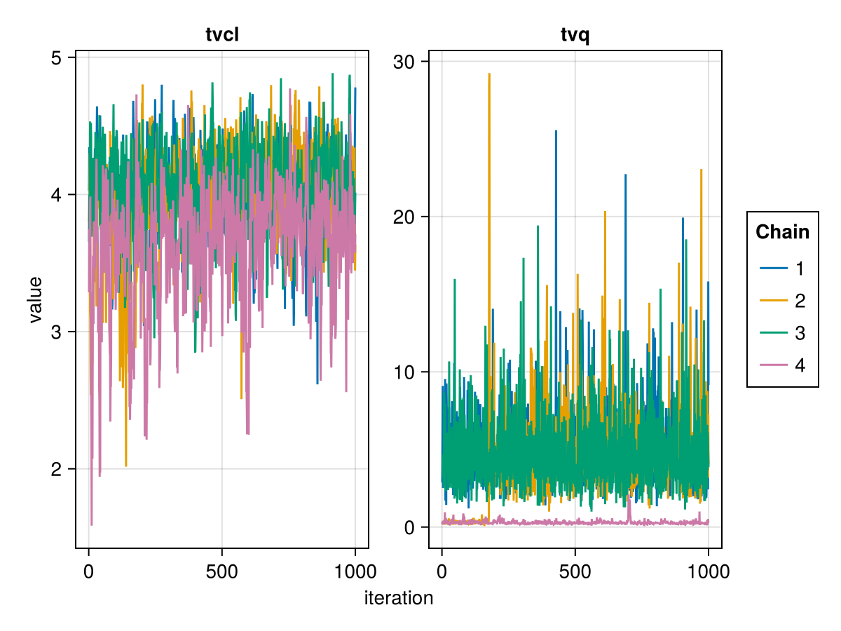
When using BayesMCMC, you can also plot the trace plots of the subject-specific parameters for a selection of subjects using:
trace_plot(tres; subjects = [1, 2])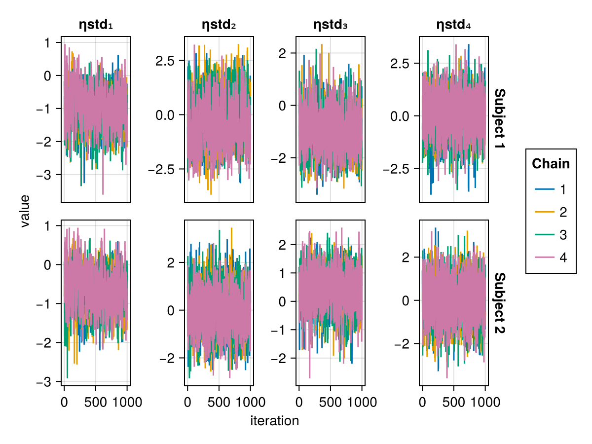
The above are examples of well mixed chains that don't indicate non-convergence.
Cumulative mean plot
The cumulative mean plot of a parameter shows the mean of the parameter value in each MCMC chain up to a certain iteration. An MCMC chain converging to a stationary posterior distribution should have the cumulative mean of each parameter converge to a fixed value. Furthermore, all the chains should be converging to the same mean for a given parameter, the posterior mean. If the cumulative mean curve is not converging or the chains are converging to different means, this is a sign of non-convergence.
PumasPlots.cummean_plot — Function
cummean_plot(results::BayesMCMCResults, kw...)Plot cumulative means for chains from BayesMCMCResults.
Keyword arguments
subjects = nothing: If set tonothing, the population parameters are plotted. If set to anIntn, the individual parameters of the nth subject are plotted. If set to anAbstractVector{<:Int}, the parameters for all chosen subjects are plotted.parameters = nothing: If set tonothing, all parameters for the chosensubjectsare plotted. If set to a vector ofSymbols, only this subset is plotted.collapse = false: If set totrue, all chains are collapsed or concatenated into one chain and plotted as such.colordim = :chain: If set to:chain, each chain is plotted in a different color. If set to:parameter, each parameter is plotted in a different color. If:chainis chosen, the different parameter values create facets, and vice versa.
Deprecated keyword arguments
linkxaxes: Can be set to:allto link all x axes, to:minimalto link only within columns, and to:noneto unlink all x axes. Pass this via AlgebraOfGraphics's genericfacetoption instead.linkyaxes: Can be set to:allto link all y axes, to:minimalto link only within rows, and to:noneto unlink all y axes. Pass this via AlgebraOfGraphics's genericfacetoption instead.
You can plot a cumulative mean plot for the population parameter :tvcl using:
cummean_plot(tres; parameters = [:tvcl])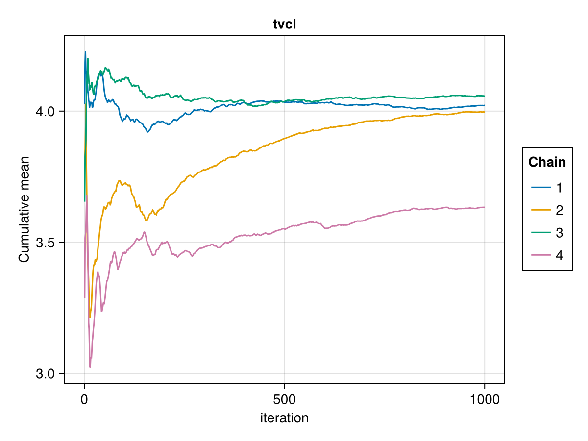
You can plot the cumulative plot of multiple parameters simultaneously by adding more parameters to the parameter names vector, e.g. [:tvq, :tvcl].
When using BayesMCMC, you can also plot the cumulative mean plots of the subject-specific parameters for a selection of subjects using:
cummean_plot(tres; subjects = [1, 2])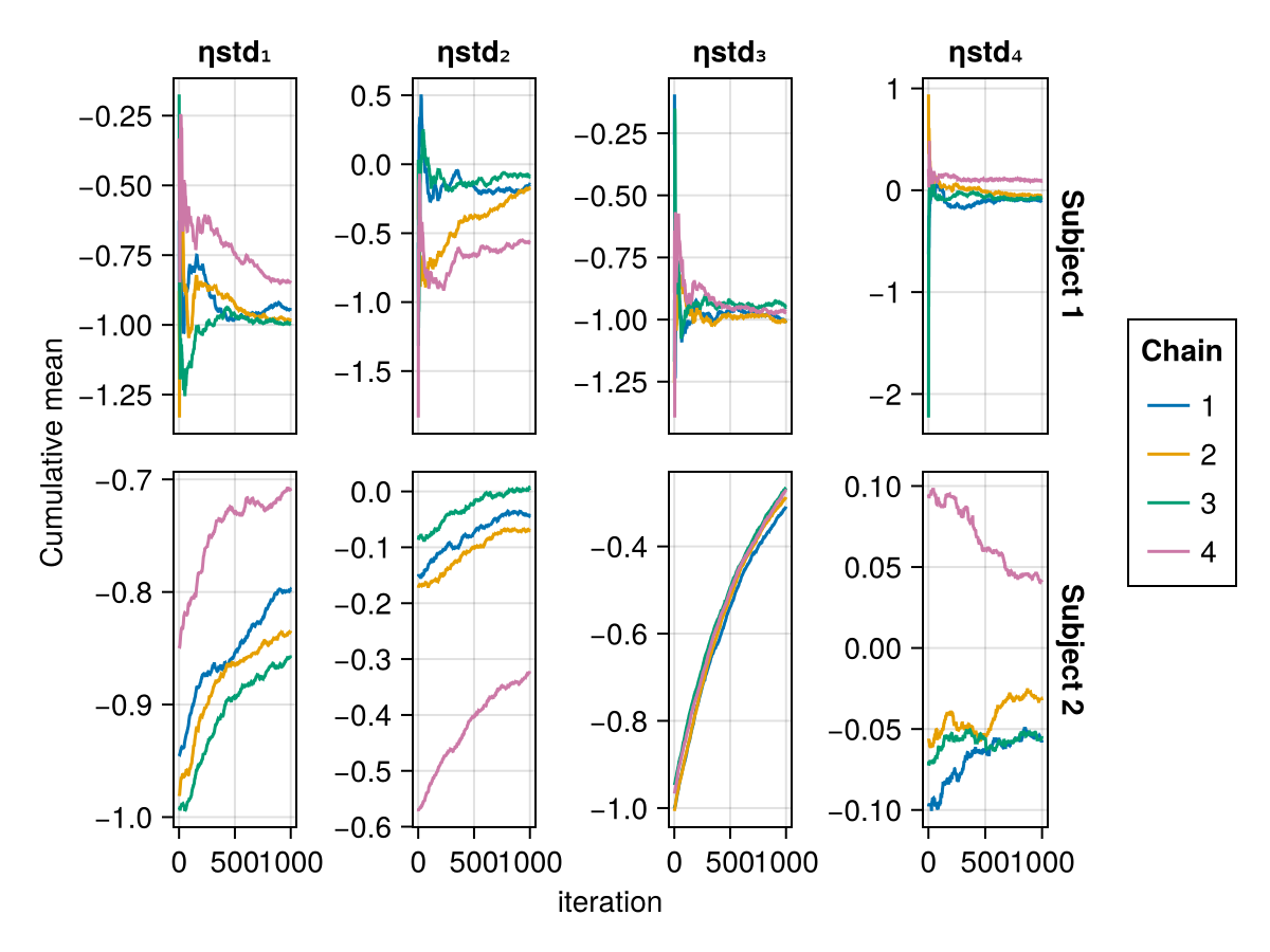
Density plot
The density plot of a parameter shows a smoothed version of the histogram of the parameter values, giving an approximate probability density function for the marginal posterior of the parameter considered. This helps us visualize the shape of the marginal posterior of each parameter.
PumasPlots.density_plot — Function
density_plot(results::BayesMCMCResults)Plot densities for chains from BayesMCMCResults.
Keyword arguments
subjects = nothing: If set tonothing, the population parameters are plotted. If set to anIntn, the individual parameters of the nth subject are plotted. If set to anAbstractVector{<:Int}, the parameters for all chosen subjects are plotted.parameters = nothing: If set tonothing, all parameters for the chosensubjectsare plotted. If set to a vector ofSymbols, only this subset is plotted.collapse = false: If set totrue, all chains are collapsed or concatenated into one chain and plotted as such.colordim = :chain: If set to:chain, each chain is plotted in a different color. If set to:parameter, each parameter is plotted in a different color. If:chainis chosen, the different parameter values create facets, and vice versa.
Deprecated keyword arguments
linkxaxes: Can be set to:allto link all x axes, to:minimalto link only within columns, and to:noneto unlink all x axes. Pass this via AlgebraOfGraphics's genericfacetoption instead.linkyaxes: Can be set to:allto link all y axes, to:minimalto link only within rows, and to:noneto unlink all y axes. Pass this via AlgebraOfGraphics's genericfacetoption instead.
You can plot a density plot for the population parameter :tvcl using:
density_plot(tres; parameters = [:tvcl])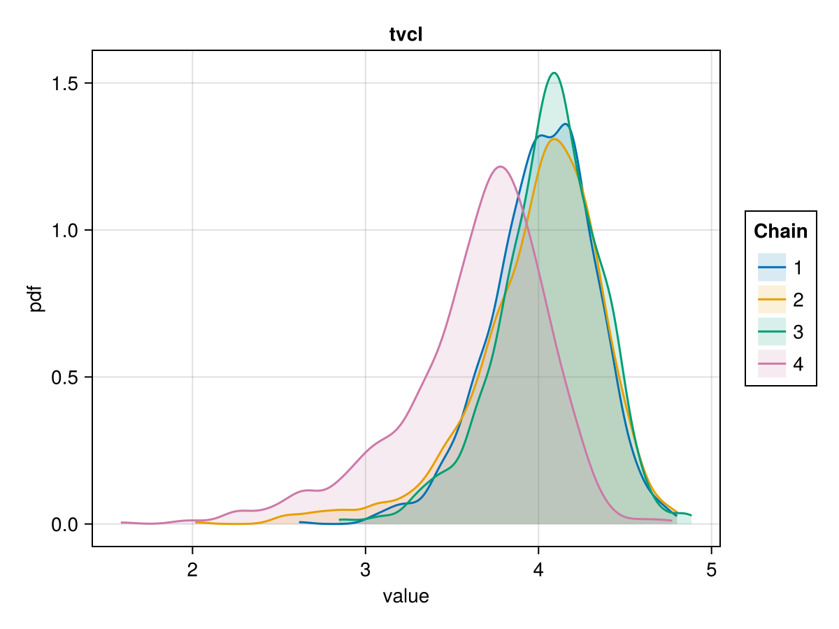
You can plot the density plots of multiple parameters simultaneously by adding more parameters to the parameter names vector, e.g. [:tvq, :tvcl].
When using BayesMCMC, you can also plot the density plots of the subject-specific parameters for a selection of subjects using:
density_plot(tres; subjects = [1, 2])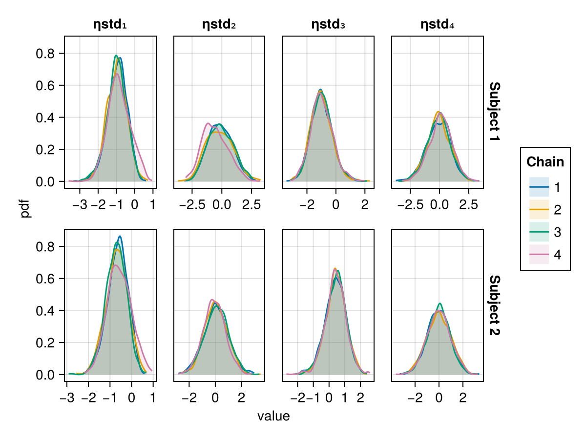
Auto-correlation plot
MCMC chains are prone to auto-correlation between the samples because each sample in the chain is a function of the previous sample. The auto-correlation plot shows the correlation between every sample with index s and the corresponding sample with index s + lag for all s ∈ 1:N-lag where N is the total number of samples. For each value of lag, we can compute a correlation measure between the samples and their lag-steps-ahead counterparts. The correlation is usually a value between 0 and 1 but can sometimes be between -1 and 0 as well. The auto-correlation plot shows the lag on the x-axis and the correlation value on the y-axis. For well behaving MCMC chains when lag increases, the corresponding correlation gets closer to 0. This means that there is less and less correlation between any 2 samples further away from each other. The value of lag where the correlation becomes close to 0 can be used to guide the thinning of the MCMC samples to extract mostly independent samples from the auto-correlated samples. The discard function can be used to perform thinning with the ratio keyword set to 1 / lag for an appropriate value of lag.
discard(tres; ratio = 1 / lag)PumasPlots.autocor_plot — Function
autocor_plot(results::BayesMCMCResults, kw...)Plot autocorrelations for chains from BayesMCMCResults.
Keyword arguments
subjects = nothing: If set tonothing, the population parameters are plotted. If set to anIntn, the individual parameters of the nth subject are plotted. If set to anAbstractVector{<:Int}, the parameters for all chosen subjects are plotted.parameters = nothing: If set tonothing, all parameters for the chosensubjectsare plotted. If set to a vector ofSymbols, only this subset is plotted.collapse = false: If set totrue, all chains are collapsed or concatenated into one chain and plotted as such.colordim = :chain: If set to:chain, each chain is plotted in a different color. If set to:parameter, each parameter is plotted in a different color. If:chainis chosen, the different parameter values create facets, and vice versa.
Deprecated keyword arguments
linkxaxes: Can be set to:allto link all x axes, to:minimalto link only within columns, and to:noneto unlink all x axes. Pass this via AlgebraOfGraphics's genericfacetoption instead.linkyaxes: Can be set to:allto link all y axes, to:minimalto link only within rows, and to:noneto unlink all y axes. Pass this via AlgebraOfGraphics's genericfacetoption instead.
You can plot an auto-correlation plot for the population parameter :tvcl using:
autocor_plot(tres; parameters = [:tvcl])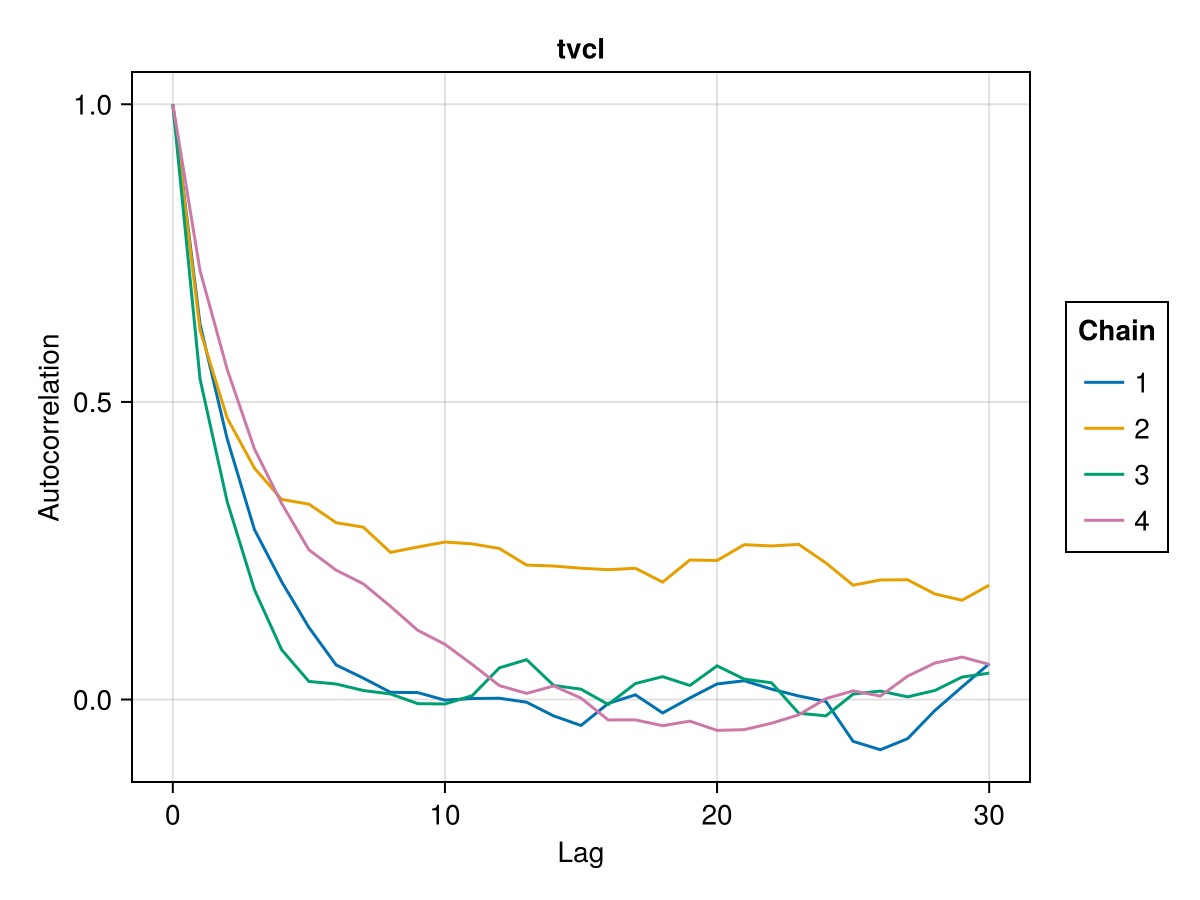
You can plot the auto-correlation plots of multiple parameters simultaneously by adding more parameters to the parameter names vector, e.g. [:tvq, :tvcl].
When using BayesMCMC, you can also plot the auto-correlation plots of the subject-specific parameters for a selection of subjects using:
autocor_plot(tres; subjects = [1, 2])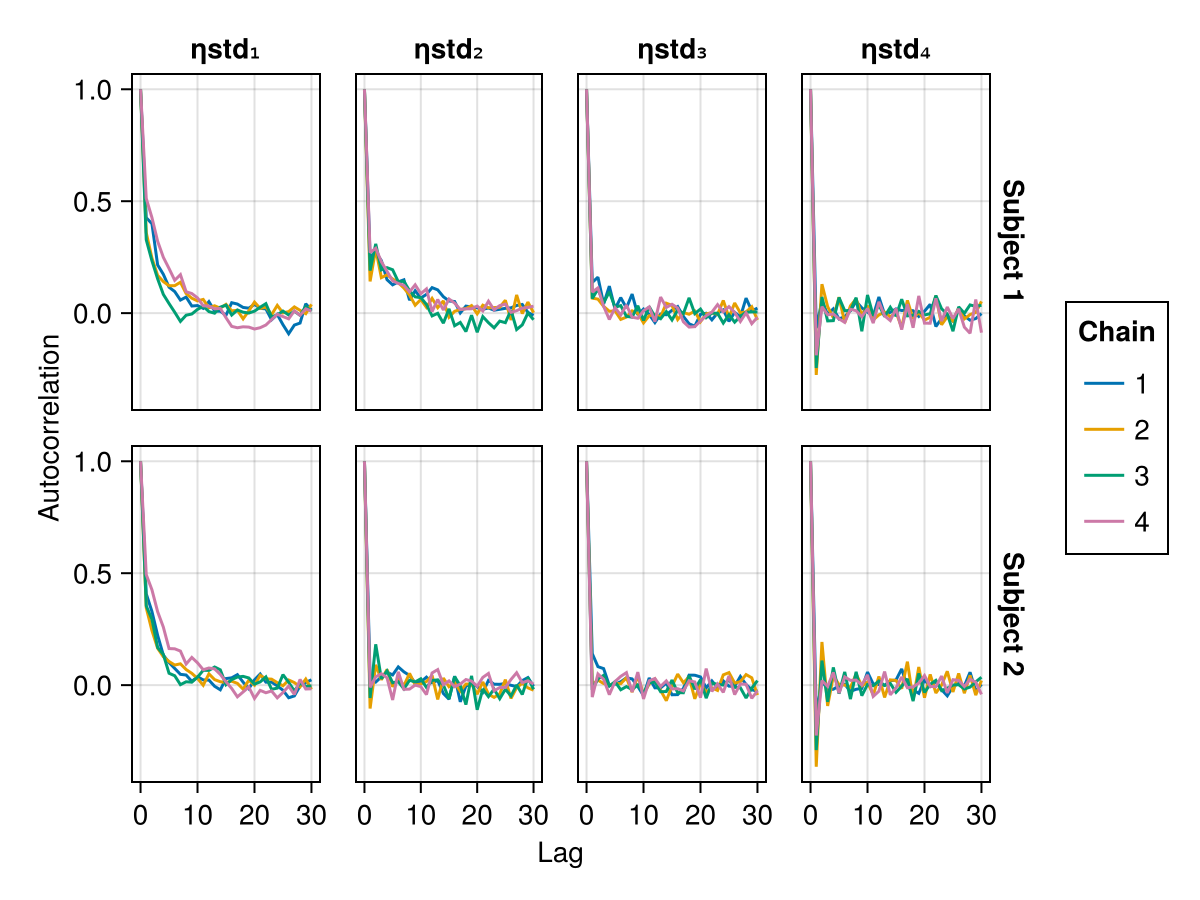
Ridge line plot
The ridge line plot shows similar information as the density plot in addition to the credible interval and quantile information.
PumasPlots.ridgeline_plot — Function
ridgeline_plot(results::BayesMCMCResults; kw...)Creates a ridgeline plot from BayesMCMCResults.
Keyword arguments
parameters = nothing: If set tonothing, all parameters for the chosensubjectare plotted. If set to a vector ofSymbols, only this subset is plotted.subject = nothing: If set tonothing, the population parameters are plotted. If set to anIntn, the individual parameters of the nth subject are plotted.hpd_val = [0.05, 0.2]: A vector of α levels for which highest posterior density intervals are plotted.q = [0.1, 0.9]: The quantile boundaries that are plotted.spacer = nothing: If set tonothing, the distance between the ridgelines is chosen using the maximum density value. You can also set this manually to aRealnumber.fill_q = true: Iftrue, only the part of the density ride between the quantiles fromqis filled. Iffalse, the whole density ridge is filled.fill_hpd = false: Iftrue, only the part of the density corresponding to the tightest hpd interval is filled.ordered = false: Iffalse, parameters are plotted in the order they have within the results struct or the by the one fromparametersif that is notnothing. Iftrue, they are plotted ordered by their median value.
You can plot a ridge line plot for the population parameter :tvcl using:
ridgeline_plot(tres; parameters = [:tvcl])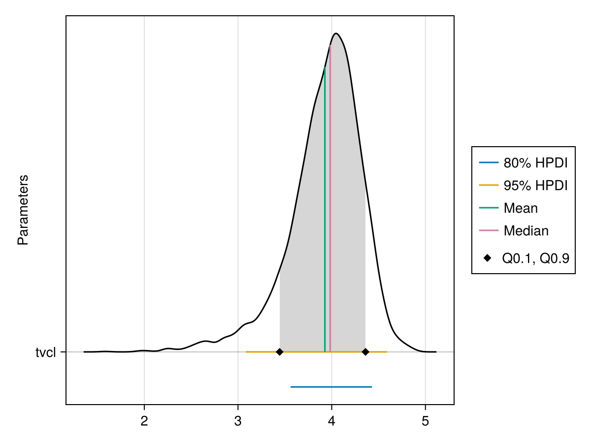
You can plot the ridge line plots of multiple parameters simultaneously by adding more parameters to the parameter names vector, e.g. [:tvq, :tvcl].
When using BayesMCMC, you can also plot the ridge line plots of the subject-specific parameters for a single subject using:
ridgeline_plot(tres; subject = 1)
Corner plot
You can plot a corner plot for the population parameters :tvvc and :tvcl using PairPlots.jl:
using PairPlots

pairplot(Chains(tres)[[:tvvc, :tvcl]])
The documentation of PairPlots.jl shows how to customize this plot further.
Chains are shown separately if passed as separate arguments to the pairplot function:
let chns = Chains(tres)[[:tvvc, :tvcl]]
    pairplot(chns[:, :, 1], chns[:, :, 2], chns[:, :, 3], chns[:, :, 4])
end
When using BayesMCMC, you can also plot the corner plot of the subject-specific parameters for a single subject using:
pairplot(Chains(tres; subject = 1))
Other diagnostics
A number of other diagnostics exist to help you identify:
- When the MCMC algorithm hasn't converged,
- How many samples to throw away as burn-in, or
- How long to run the MCMC for.
Geweke diagnostic
MCMCDiagnosticTools.gewekediag — Method
gewekediag(b::BayesMCMCResults; subject::Union{Nothing,Int} = nothing, first::Real = 0.1, last::Real = 0.5)Computes the Geweke diagnostic [Geweke1991] for each chain outputting a p-value per parameter. If subject is nothing (default), the chains diagnosed are those of the population parameters. If subject is set to an integer index, the chains diagnosed are those of the subject-specific parameters corresponding to the subject with the input index.
The Geweke diagnostic compares the sample means of two disjoint sub-chains X₁ and X₂ of the entire chain using a normal difference of means hypothesis test where the null and alternative hypotheses are defined as:
H₀: μ₁ = μ₂H₁: μ₁ ≂̸ μ₂whereμ₁andμ₂are the population means. The first sub-chainX₁is taken as the first(first * 100)% of the samples in the chain, wherefirstis a keyword argument defaulting to0.1. The second sub-chainX₂is taken as the last(last * 100)% of the samples in the chain, wherelastis a keyword argument defaulting to0.5.
The test statistic used is: z₀ = x̅₁ - x̅₂ / √(s₁² + s₂²) where x̅₁ and x̅₂ are the sample means of X₁ and X₂ respectively, and s₁ and s₂ are the Markov Chain standard error (MCSE) estimates of X₁ and X₂ respectively. Auto-correlation is assumed within the samples of each individual sub-chain, but the samples in X₁ are assumed to be independent of the samples in X₂. The p-value output is an estimate of P(|z| > |z₀|), where z is a standard normally distributed random variable.
Low p-values indicate one of the following:
- The first and last parts of the chain are sampled from distributions with different means, i.e. non-convergence,
- The need to discard some initial samples as burn-in, or
- The need to run the sampling for longer due to lack of samples or high auto-correlation.
High p-values indicate the inability to conclude that the means of the first and last parts of the chain are different with statistical significance. However, this alone does not guarantee convergence to a fixed posterior distribution because:
- Either the standard deviations or higher moments of
X₁andX₂may be different, or - The independence assumption between
X₁andX₂may not be satisfied when high auto-correlation exists.
Heidelberger and Welch diagnostic
MCMCDiagnosticTools.heideldiag — Method
heideldiag(b::BayesMCMCResults; subject::Union{Nothing,Int} = nothing, alpha::Real = 0.05, eps::Real = 0.1, start::Integer = 1)Compute the Heidelberger and Welch diagnostic [Heidelberger1983] for each chain. If subject is nothing (default), the chains diagnosed are those of the population parameters. If subject is set to an integer index, the chains diagnosed are those of the subject-specific parameters corresponding to the subject with the input index.
The Heidelberger diagnostic attempts to:
- Identify a cutoff point for the initial transient phase for each parameter, after which the samples can be assumed to come from a steady-state posterior distribution. The initial transient phase can be removed as burn-in. The cutoff point for each parameter is given in the
burnincolumn of the output dataframe. - Estimate the relative confidence interval (confidence interval divided by the mean) for the mean of the steady-state posterior distribution of each parameter, assuming such steady-state distribution exists in the samples. A large confidence interval implies either the lack of convergence to a stationary distribution or lack of samples. Half the relative confidence interval is given in the
halfwidthcolumn of the output dataframe. Thetestcolumn will betrue(1) if thehalfwidthis less than the input targeteps(default is 0.1) andfalse(0) otherwise. Note that parameters with mean value close to 0 can have erroneous relative confidence intervals because of the division by the mean. Thetestvalue can therefore be expected to befalse(0) for those parameters without concluding lack of convergence. - Quantify the extent to which the distribution of the samples is stationary using statistical testing. The returned p-value, shown in the
pvaluecolumn of the output dataframe, can be considered a measure of mean stationarity. A p-value lower than the input thresholdalpha(default is 0.05) implies lack of stationarity of the mean, i.e. the posterior samples did not converge to a steady-state distribution with a fixed mean.
The Heidelberger diagnostic only tests for the mean of the distribution. Therefore, it can only be used to detect lack of convergence and not to prove convergence. In other words, even if all the numbers seem normal, one cannot conclude that the chain converged to a stationary distribution or that it converged to the true posterior.
Raftery and Lewis diagnostic
MCMCDiagnosticTools.rafterydiag — Method
rafterydiag(b::BayesMCMCResults; subject::Union{Nothing,Int} = nothing, q = 0.025, r = 0.005, s = 0.95, eps = 0.001)Compute the Raftery and Lewis diagnostic [Raftery1992]. This diagnostic is used to determine the number of iterations required to estimate a specified quantile q within a desired degree of accuracy. The diagnostic is designed to determine the number of autocorrelated samples required to estimate a specified quantile $\theta_q$, such that $\Pr(\theta \le \theta_q) = q$, within a desired degree of accuracy. In particular, if $\hat{\theta}_q$ is the estimand and $\Pr(\theta \le \hat{\theta}_q) = \hat{P}_q$ the estimated cumulative probability, then accuracy is specified in terms of r and s, where $\Pr(q - r < \hat{P}_q < q + r) = s$. Thinning may be employed in the calculation of the diagnostic to satisfy its underlying assumptions. However, users may not want to apply the same (or any) thinning when estimating posterior summary statistics because doing so results in a loss of information. Accordingly, sample sizes estimated by the diagnostic tend to be conservative (too large).
Furthermore, the argument r specifies the margin of error for estimated cumulative probabilities and s the probability for the margin of error. eps specifies the tolerance within which the probabilities of transitioning from initial to retained iterations are within the equilibrium probabilities for the chain. This argument determines the number of samples to discard as a burn-in sequence and is typically left at its default value.
Posterior queries
Summary statistics
There are a number of functions you can call on the output of the fit or discard function. Assume res is the output from fit. You can use the get_params function to get a vector of posterior samples of the population parameter.
When using BayesMCMC, you can further get the posterior samples of the subject-specific parameters using:
get_randeffs(res, subject_ind)where subject_ind is an integer of the subject index in the fit training population.
You can compute summary statistics of the posterior samples using the summarystats function.
summarystats(tres)Summary Statistics
parameters mean std mcse ess_bulk ess_tail rhat ess_per_sec
Symbol Float64 Float64 Float64 Float64 Float64 Float64 Float64
tvcl 3.9274 0.3908 0.0673 35.9857 138.4455 1.1393 0.0259
tvq 3.5771 3.0201 0.7276 14.6568 83.0172 1.4640 0.0106
tvvc 58.2299 6.7064 0.7550 76.2769 173.8406 1.0677 0.0549
tvvp 47.1652 73.7817 20.8094 15.1117 80.3076 1.4391 0.0109
σ 0.2360 0.0124 0.0002 2568.0946 3015.4781 1.0076 1.8492
C₂,₁ -0.0530 0.4469 0.0417 115.3075 1070.5141 1.0448 0.0830
C₃,₁ 0.5431 0.2059 0.0050 1510.2194 1693.7128 1.0027 1.0875
C₄,₁ -0.0132 0.4434 0.0216 385.6855 2299.6459 1.0183 0.2777
C₃,₂ 0.0203 0.4536 0.0188 588.8355 1620.0843 1.0033 0.4240
C₄,₂ 0.0089 0.4566 0.0075 3692.0481 3060.4675 1.0013 2.6585
C₄,₃ -0.0483 0.4444 0.0066 4424.5188 3297.7383 1.0024 3.1860
ω₁ 0.2353 0.0725 0.0039 301.3624 1028.3267 1.0240 0.2170
ω₂ 0.3279 0.2593 0.0069 1547.3103 1801.6850 1.0024 1.1142
ω₃ 0.3384 0.0826 0.0028 401.0084 1928.0716 1.0184 0.2888
ω₄ 0.2605 0.2192 0.0149 420.6692 455.2127 1.0254 0.3029
summarystats(tres; subjects = 1)Summary Statistics
parameters mean std mcse ess_bulk ess_tail rhat ess_per_sec
Symbol Float64 Float64 Float64 Float64 Float64 Float64 Float64
tvcl 3.9274 0.3908 0.0673 35.9857 138.4455 1.1393 0.0259
tvq 3.5771 3.0201 0.7276 14.6568 83.0172 1.4640 0.0106
tvvc 58.2299 6.7064 0.7550 76.2769 173.8406 1.0677 0.0549
tvvp 47.1652 73.7817 20.8094 15.1117 80.3076 1.4391 0.0109
σ 0.2360 0.0124 0.0002 2568.0946 3015.4781 1.0076 1.8492
C₂,₁ -0.0530 0.4469 0.0417 115.3075 1070.5141 1.0448 0.0830
C₃,₁ 0.5431 0.2059 0.0050 1510.2194 1693.7128 1.0027 1.0875
C₄,₁ -0.0132 0.4434 0.0216 385.6855 2299.6459 1.0183 0.2777
C₃,₂ 0.0203 0.4536 0.0188 588.8355 1620.0843 1.0033 0.4240
C₄,₂ 0.0089 0.4566 0.0075 3692.0481 3060.4675 1.0013 2.6585
C₄,₃ -0.0483 0.4444 0.0066 4424.5188 3297.7383 1.0024 3.1860
ω₁ 0.2353 0.0725 0.0039 301.3624 1028.3267 1.0240 0.2170
ω₂ 0.3279 0.2593 0.0069 1547.3103 1801.6850 1.0024 1.1142
ω₃ 0.3384 0.0826 0.0028 401.0084 1928.0716 1.0184 0.2888
ω₄ 0.2605 0.2192 0.0149 420.6692 455.2127 1.0254 0.3029
This includes information about the mean, standard deviation, Monte Carlo standard error (MCSE), ESS, $\widehat{R}$ and ESS per second.
You can find the probability of certain binary outcomes of the posterior samples using the mean function. For example, the following computes the probability that the population parameter p.tvcl is less than 4.
mean(tres) do p
    p.tvcl < 4
end0.5205The following can be used to compute the probability that the subject-specific parameter ηstd[2] for subject 1 is less than or equal to 0:
mean(tres; subject = 1) do p
    p.ηstd[2] <= 0
end0.59725You can replace the binary outcome c.ηstd[2] < 0 with an arbitrary function of the parameters. For example, if C was a correlation matrix parameter, and you want the mean of the lower triangular Cholesky factors of the C samples, you can do:
mean(tres) do p
    cholesky(p.C).L
end
4×4 Matrix{Float64}:
1.0 0.0 0.0 0.0
-0.0530042 0.881326 0.0 0.0
0.543132 0.0598836 0.668042 0.0
-0.0131772 0.0177949 -0.0412598 0.581827You can call the cor function on tres to get a correlation DataFrame of the population parameters:
cor(tres)Correlation
parameters tvcl tvq tvvc tvvp σ C₂,₁ C₃,₁ C₄,₁ C₃,₂ C₄,₂ ⋯
Symbol Float64 Float64 Float64 Float64 Float64 Float64 Float64 Float64 Float64 Float64 Flo ⋯
tvcl 1.0000 0.3530 0.3091 -0.4378 -0.0446 0.2586 -0.2874 -0.0680 0.0890 0.0416 -0. ⋯
tvq 0.3530 1.0000 -0.2980 -0.5744 -0.0685 0.2082 -0.0351 -0.1311 -0.0017 0.0088 -0. ⋯
tvvc 0.3091 -0.2980 1.0000 0.2873 0.0510 -0.0423 -0.3331 0.1017 0.1120 -0.0279 0. ⋯
tvvp -0.4378 -0.5744 0.2873 1.0000 0.0719 -0.2437 0.0385 0.1457 -0.0015 -0.0182 0. ⋯
σ -0.0446 -0.0685 0.0510 0.0719 1.0000 -0.0267 -0.0070 0.0106 0.0052 0.0057 -0. ⋯
C₂,₁ 0.2586 0.2082 -0.0423 -0.2437 -0.0267 1.0000 -0.0373 -0.0338 0.5025 -0.0386 -0. ⋯
C₃,₁ -0.2874 -0.0351 -0.3331 0.0385 -0.0070 -0.0373 1.0000 -0.0460 -0.0865 0.0056 -0. ⋯
C₄,₁ -0.0680 -0.1311 0.1017 0.1457 0.0106 -0.0338 -0.0460 1.0000 0.0038 -0.0785 0. ⋯
C₃,₂ 0.0890 -0.0017 0.1120 -0.0015 0.0052 0.5025 -0.0865 0.0038 1.0000 -0.0433 -0. ⋯
C₄,₂ 0.0416 0.0088 -0.0279 -0.0182 0.0057 -0.0386 0.0056 -0.0785 -0.0433 1.0000 0. ⋯
C₄,₃ -0.0189 -0.0241 0.0722 0.0468 -0.0241 -0.0222 -0.0003 0.5290 -0.0170 0.0001 1. ⋯
ω₁ -0.6816 -0.1460 -0.2699 0.1719 -0.0107 -0.1793 0.3094 0.0651 -0.1066 -0.0275 0. ⋯
ω₂ -0.1788 -0.0201 -0.0317 0.0089 0.0130 -0.1481 0.0160 0.0234 0.0149 -0.0081 0. ⋯
ω₃ -0.2002 0.1105 -0.5511 -0.1298 -0.0746 0.0168 0.3198 -0.0621 -0.1007 0.0177 -0. ⋯
ω₄ -0.1809 -0.1565 0.0759 0.1812 0.0429 -0.0916 0.0500 0.0318 -0.0214 -0.0059 -0. ⋯
5 columns omitted
To get the correlations of the subject-specific parameters for subject 1, you can use:
cor(tres; subjects = 1)Correlation
parameters tvcl tvq tvvc tvvp σ C₂,₁ C₃,₁ C₄,₁ C₃,₂ C₄,₂ ⋯
Symbol Float64 Float64 Float64 Float64 Float64 Float64 Float64 Float64 Float64 Float64 Flo ⋯
tvcl 1.0000 0.3530 0.3091 -0.4378 -0.0446 0.2586 -0.2874 -0.0680 0.0890 0.0416 -0. ⋯
tvq 0.3530 1.0000 -0.2980 -0.5744 -0.0685 0.2082 -0.0351 -0.1311 -0.0017 0.0088 -0. ⋯
tvvc 0.3091 -0.2980 1.0000 0.2873 0.0510 -0.0423 -0.3331 0.1017 0.1120 -0.0279 0. ⋯
tvvp -0.4378 -0.5744 0.2873 1.0000 0.0719 -0.2437 0.0385 0.1457 -0.0015 -0.0182 0. ⋯
σ -0.0446 -0.0685 0.0510 0.0719 1.0000 -0.0267 -0.0070 0.0106 0.0052 0.0057 -0. ⋯
C₂,₁ 0.2586 0.2082 -0.0423 -0.2437 -0.0267 1.0000 -0.0373 -0.0338 0.5025 -0.0386 -0. ⋯
C₃,₁ -0.2874 -0.0351 -0.3331 0.0385 -0.0070 -0.0373 1.0000 -0.0460 -0.0865 0.0056 -0. ⋯
C₄,₁ -0.0680 -0.1311 0.1017 0.1457 0.0106 -0.0338 -0.0460 1.0000 0.0038 -0.0785 0. ⋯
C₃,₂ 0.0890 -0.0017 0.1120 -0.0015 0.0052 0.5025 -0.0865 0.0038 1.0000 -0.0433 -0. ⋯
C₄,₂ 0.0416 0.0088 -0.0279 -0.0182 0.0057 -0.0386 0.0056 -0.0785 -0.0433 1.0000 0. ⋯
C₄,₃ -0.0189 -0.0241 0.0722 0.0468 -0.0241 -0.0222 -0.0003 0.5290 -0.0170 0.0001 1. ⋯
ω₁ -0.6816 -0.1460 -0.2699 0.1719 -0.0107 -0.1793 0.3094 0.0651 -0.1066 -0.0275 0. ⋯
ω₂ -0.1788 -0.0201 -0.0317 0.0089 0.0130 -0.1481 0.0160 0.0234 0.0149 -0.0081 0. ⋯
ω₃ -0.2002 0.1105 -0.5511 -0.1298 -0.0746 0.0168 0.3198 -0.0621 -0.1007 0.0177 -0. ⋯
ω₄ -0.1809 -0.1565 0.0759 0.1812 0.0429 -0.0916 0.0500 0.0318 -0.0214 -0.0059 -0. ⋯
5 columns omitted
Credible intervals
The credible interval with a target probability $p$ of a parameter is any interval that has a probability mass of approximately $p$ according to the posterior distribution. That is the probability that the parameter value is in this interval according to the posterior distribution should be $\approx p$. There are 2 main ways to define the credible interval. The first is using quantiles. Say the target probability is 95%. The interval from the 2.5% quantile to the 97.5% quantile is an interval where 95% of the posterior samples lie, hence it has approximately 95% probability mass. You can do this in Pumas using:
quantile(tres; q = [0.025, 0.975])Quantiles
parameters 2.5% 97.5%
Symbol Float64 Float64
tvcl 2.9569 4.5341
tvq 0.1765 10.1853
tvvc 44.5772 71.2101
tvvp 4.5428 247.9452
σ 0.2125 0.2616
C₂,₁ -0.8460 0.7851
C₃,₁ 0.0535 0.8566
C₄,₁ -0.8131 0.8025
C₃,₂ -0.8104 0.8237
C₄,₂ -0.8198 0.8155
C₄,₃ -0.8260 0.7890
ω₁ 0.1389 0.4172
ω₂ 0.0148 0.9435
ω₃ 0.2155 0.5379
ω₄ 0.0083 0.8198
to get the 2.5% and 97.5% quantiles of all the population parameters.
However, using quantiles is generally going to lead to a wider than necessary interval unless the posterior probability density function is symmetric around the median. In other words, we can often find smaller intervals that still has the same target probability mass of 95%. Such an interval is often known as the highest probability density (HPD) interval. You can get the HPD interval for the 95% target probability using the hpd function in Pumas:
hpd(tres; alpha = 1 - 0.95)HPD
parameters lower upper
Symbol Float64 Float64
tvcl 3.0869 4.5907
tvq 0.1245 8.7188
tvvc 45.1716 71.4403
tvvp 2.8433 200.0630
σ 0.2102 0.2585
C₂,₁ -0.8721 0.7470
C₃,₁ 0.1493 0.8971
C₄,₁ -0.8185 0.7895
C₃,₂ -0.8162 0.8143
C₄,₂ -0.8022 0.8326
C₄,₃ -0.8476 0.7532
ω₁ 0.1245 0.3759
ω₂ 0.0006 0.8414
ω₃ 0.1946 0.4974
ω₄ 0.0000 0.6937
Using the HPD interval as the credible interval is generally preferred over the quantile method.
Simulate from the posterior
You can simulate the model under samples from the posterior using the simobs function as such:
sims = mapreduce(
    i -> simobs(poppk2cpt, fit_pop[i], sample(tres, 10; subject = i)...),
    vcat,
    1:length(fit_pop),
)
Simulated population (Vector{<:Subject})
Simulated subjects: 150
Simulated variables: dvThis generates 10 samples from the posterior and simulates the model for each subject in the training data. The output is 15 sets of simulations with 10 replications for each subject concatenated into one 150 element vector sims. The resulting simulations will contain all the simulated intermediate quantities from the model, e.g. the @pre block variables and @dynamics solution. If we had used map without the vcat reducer, we would have gotten a vector of 15 elements where each element is a vector of 10 simulations for each subject.
Keep in mind, that the simulation of the dependent variables with simobs is performed by sampling from the error model in the @derived block due to the default keyword setting of simulate_error = true. To simply return the expected value of the error distribution (simulate_error = false) which gives you a distribution of predictions, aka the posterior predictive distribution. See also the predict function for an alternative way of calculating predictions.
To simulate for an individual subject with index subject_ind, you can use the following instead:
subject_ind = 1
fixed_sample_1, randeffs_sample_1 = sample(tres, 10; subject = subject_ind)
sims = simobs(poppk2cpt, fit_pop[subject_ind], fixed_sample_1, randeffs_sample_1)
Simulated population (Vector{<:Subject})
Simulated subjects: 10
Simulated variables: dvOther keyword arguments you can specify include:
diffeq_options: aNamedTupleof all the differential equations solver's keyword arguments such asalg,abstol, andreltol. See the DifferentialEquations documentation for more details.rng: the random number generator used during MCMC. This can be used for reproducibility.obstimes: The time points to simulate at. This defaults to the observation times of the individual subjects if unset.
After simulating, the result sims can then be inspected using a visual predictive check (VPC) plot as such:
vpc_res = vpc(sims)

using PumasUtilities
vpc_plot(vpc_res)
To use vpc_plot, you will need to load the PumasUtilities package by calling using PumasUtilities once as shown above. The following is a VPC plot for the first subject, obtained using:
using PumasUtilities
fixed_sample_first, randeffs_sample_first = sample(tres, 10; subject = 1)
sims = simobs(poppk2cpt, fit_pop[1], fixed_sample_first, randeffs_sample_first)
vpc_res = vpc(sims)
vpc_plot(vpc_res)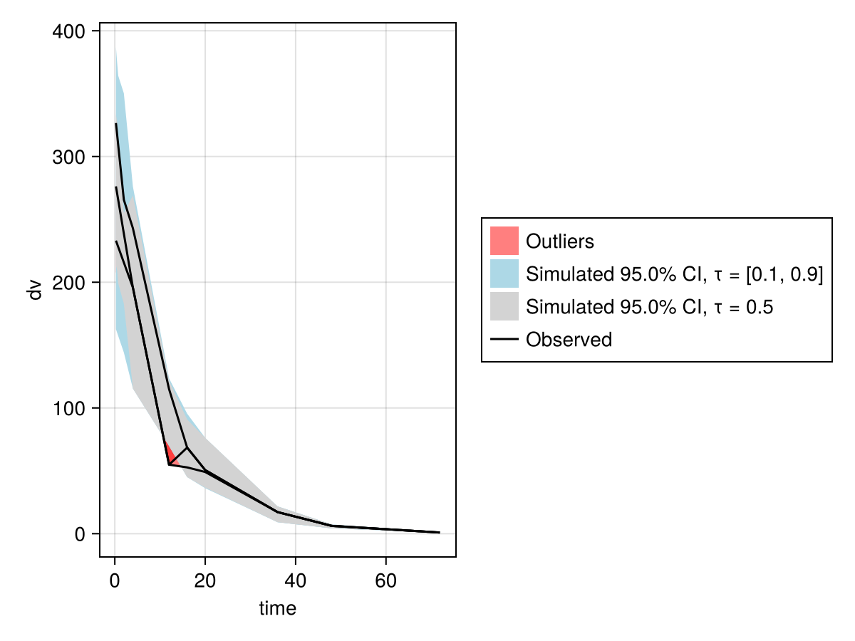
The result from simobs can be further queried using the postprocess function which you can learn more about from the Post-processing simulations section in the Simulations documentation.
Cross-validation and model selection
Background
In the Bayesian workflow, it is common to evaluate and compare models using their predictive power for out-of-sample data. One popular model evaluation metric for out-of-sample prediction accuracy is the so-called expected log predictive density (ELPD). Let $\mathcal{M}$ be a model with parameters $\theta \in \Theta$ that describes the data generating process of the observed data $y$. The ELPD is defined as:
\[\begin{align} \text{ELPD} = \int_{y_{pred}} \log p(y_{pred} | y, \mathcal{M}) p_t(y_{pred}) dy_{pred} \end{align}\]
where $y_{pred}$ is unobserved data, $p_t(y_{pred})$ is the true data generating distribution of $y_{pred}$ (unknown in practice) and $p(y_{pred} | y, \mathcal{M})$ is the posterior predictive density defined as:
\[\begin{align} p(y_{pred} | y, \mathcal{M}) = \int_{\Theta} p(y_{pred} | \theta, \mathcal{M}) p(\theta | y, \mathcal{M}) d\theta \end{align}\]
where $p(\theta | y, \mathcal{M})$ describes the posterior distribution of $\theta$ given the observed data $y$ and the model $\mathcal{M}$. Since the true data generating distribution is unknown, it is common to approximate ELPD by an empirical distribution over the observed data. One such estimator is the log pointwise predictive density (lppd). Let $y_i$ be the $i^{th}$ observation and $\theta^{[j]}$ be the $j^{th}$ sample draw from the posterior $p(\theta | y, \mathcal{M})$. The lppd can be calculated using:
\[\begin{align} \text{lppd} & = \frac{1}{N} \sum_{i=1}^N \log p(y_i | y, \mathcal{M}) \\ & = \frac{1}{N} \sum_{i=1}^N \log \int_{\Theta} p(y_i | \theta, \mathcal{M}) p(\theta | y, \mathcal{M}) d\theta \\ & \approx \frac{1}{N} \sum_{i=1}^N \log \Big( \frac{1}{M} \sum_{j=1}^M p(y_i | \theta^{[j]}, \mathcal{M}) \Big) \end{align}\]
A shortcoming of the lppd is that it is not representative of predictive accuracy on unseen data, since $y_i$ is used both for inference on the posterior and to evaluate the model out-of-sample.
Leave-k-out cross-validation
Cross-validation overcomes this problem by ensuring that $y_i$ is not used for inference on the posterior when evaluating the out-of-sample performance for $y_i$. The simplest way to divide the data into in-sample and out-of-sample subsets is the leave-one-out (loo) cross-validation where in each outer iteration, one data point is considered out-of-sample and the remaining are in-sample. The leave-one-out, log predictive density (loo-lpd) is defined as:
\[\begin{align} \text{loo-lpd} & = \frac{1}{N} \sum_{i=1}^N \log p(y_i | y_{-i}, \mathcal{M}) \\ & = \frac{1}{N} \sum_{i=1}^N \log \int_{\Theta} p(y_i | \theta, \mathcal{M}) p(\theta | y_{-i}, \mathcal{M}) d\theta \\ & \approx \frac{1}{N} \sum_{i=1}^N \log \Big( \frac{1}{M} \sum_{j=1}^M p(y_i | \theta^{[j]}_{\backslash i}, \mathcal{M}) \Big) \end{align}\]
where $y_{-i}$ is all data excluding $y_i$ and $\theta^{[j]}_{\backslash i}$ is the $j^{th}$ draw of a sample from the posterior $p(\theta | y_{-i}, \mathcal{M})$. This can be generalized to leave $k$-out cross validation where $y_i$ is replaced with a vector of observations of length $k$.
Leave-future-k-out cross-validation
When working with time-series data, it can often be more useful to evaluate models based on their ability to predict future values using nothing but past values for training. This gives rise to another variant of cross-validation called leave-future-one-out (lfoo) cross-validation and the lfoo-lpd which is defined as:
\[\begin{align} \text{lfoo-lpd} & = \frac{1}{N - t} \sum_{i=t+1}^N \log p(y_i | y_{1:i-1}, \mathcal{M}) \\ & = \frac{1}{N - t} \sum_{i=t+1}^N \log \int_{\Theta} p(y_i | \theta, \mathcal{M}) p(\theta | y_{1:i-1}, \mathcal{M}) d\theta \\ & \approx \frac{1}{N - t} \sum_{i=t+1}^N \log \Big( \frac{1}{M} \sum_{j=1}^M p(y_i | \theta^{[j]}_{\backslash i:N}, \mathcal{M}) \Big) \end{align}\]
where $t$ is the minimum number of data points used for training/inference, $y_{1:i-1}$ is the past data up to point $i - 1$ and $\theta^{[j]}_{\backslash i:N}$ is the $j^{th}$ draw of a sample from the posterior $p(\theta | y_{1:i-1}, \mathcal{M})$ obtained by excluding the points $y_{i:N}$ from the inference.
Cross-validation for hierarchical models
When performing cross-validation in a hierarchical model, there are multiple ways to measure the predictive power of the model. For instance in hierarchical PKPD modeling, the goal is to learn a population model to make predictions on new patients while simultaneously learning subject-specific models to make future predictions for specific subjects having seen their past response to drugs. These models are useful for dose selection and dose adaptation for new or existing patients with the objective of maximizing the therapeutic effect while avoiding toxicity.
Depending on the prediction task of interest, one may choose to treat each time observation as a data point or each entire patient/subject as a data point. If the goal is to evaluate the model's ability to predict responses for new patients, leave-one-subject-out or leave-one-future-subject-out cross-validation should be used. Alternatively, if the goal is to evaluate the model's ability to predict future drug concentrations or any other observable time-dependent quantity the model predicts, then leaving future observations out for each subject makes more sense. This will be called leave-one-observation-out or leave-one-future-observation-out cross-validation.
The choice of what constitutes a point to leave out when doing cross-validation affects the way the predictive likelihoods are computed:
\[\begin{align} p(y_i | \theta^{[j]}, \mathcal{M}) \end{align}\]
When leaving subjects out, we are often interested in the marginal likelihood of this subject given a posterior draw of the population parameters, marginalizing out the subject-specific parameters. Alternatively, the conditional likelihood can also be used for some default or typical values of the subject-specific parameters, e.g. the mode of the prior distribution. To marginalize subject-specific parameters, approximate integration methods such as LaplaceI and FOCE can be used to obtain the marginal likelihood.
On the other hand when leaving observations out in a single subject, the quantity of interest is often the conditional likelihood given each draw from the joint posterior of population and subject-specific parameters of individual subjects given previous data of the subject.
Pareto smoothed importance sampling cross-validation
Evaluating the loo-lpd or lfoo-lpd is expensive since one needs to draw samples from $N$ or $N - t$ different posteriors, e.g. from $p(\theta | y_{-i}, \mathcal{M})$ for $i=1,\dots,N$. Typically, this will be done by MCMC, e.g. the NUTS algorithm, which in spite of recent progress, remain computationally expensive when the number of parameters is large and the curvature of the posterior is uneven along one or more dimensions.
One approach to overcome this difficulty, is the Pareto-smoothed importance sampling method for leave-one-out, cross-validation (PSIS-LOO-CV). In PSIS-LOO-CV, MCMC is run only once on the full data. The same samples are then re-used in each outer iteration of CV but using different weights. The weights are determined using importance sampling (IS) by comparing the likelihood with one data point left out to the likelihood of the full dataset. The raw importance weights are then smoothed by fitting them to a generalized Pareto distribution. The smoothed weights can then be used to estimate the ELPD contribution of each data point.
Beside the ability to approximate the ELPD, PSIS-LOO-CV also provides a useful diagnostic which is the shape parameter of the Pareto distribution fitted to the raw weights when leaving out each data point. Data points that when removed lead to a large shape parameter are more influential than data points which have a low shape parameter. For highly influential points where the Pareto shape parameter is higher than 0.7, the ELPD contribution for this point can be considered unreliable. In those cases, resampling from the posterior after removing the influential point is recommended instead of relying on PSIS-LOO-CV.
Cross-validation in Pumas
You can do almost all types of cross-validation for hierarchical models using Pumas. The main function that performs cross-validation in Pumas is the crossvalidate function.
There are 2 families of the cross-validation algorithms available in Pumas:
- Resampling-based CV which performs the MCMC again for each data point or subset left out. This algorithm is constructed using the
ExactCrossvalidationstruct. - PSIS-based CV which uses the importance sampling and weight smoothing approach to avoid the need for resampling. This algorithm is constructed using the
PSISCrossvalidationstruct.
Pumas.crossvalidate — Function
crossvalidate(b::BayesMCMCResults, cv_method::ExactCrossvalidation)Runs cross-validation by re-running the MCMC sampling while leaving out some data points each time. The first argument b is the output of the MCMC fit. The choice of how the data is split in each run is specified in the cv_method argument which is an instance of ExactCrossvalidation. Please refer to the documentation of ExactCrossvalidation by typing ?ExactCrossvalidation for details on the parameters of the method.
crossvalidate(b::BayesMCMCResults, cv_method::PSISCrossvalidation)Performs cross-validation using the Pareto smoothed importance sampling (PSIS) approach by re-weighing the samples while leaving out some data points each time. The first argument b is the output of the MCMC fit. The choice of how the data is split in each run is specified in the cv_method argument which is an instance of PSISCrossvalidation.
The constructor for a resampling-based CV method is
Pumas.ExactCrossvalidation — Type
ExactCrossvalidation(; split_method, split_by, ensemblealg)Defines an instance of the ExactCrossvalidation algorithm for crossvalidation. In this algorithm, the fitting is re-run while leaving out a subset of the data each time.
The way by which the data is split between training and validation sets is determined using the keyword arguments split_method and split_by. The split_method argument can be of any of the following types:
LeaveKfor leave-K-out cross-validationKFoldfor K-fold cross-validationLeaveFutureKfor leaving K future points at a time
while split_by can be of any of the following types:
BySubjectfor leaving out subjectsByObservationfor leaving out individual observations per subject
Please refer to the documentation of each of the above types for the parameters of each split method, e.g. typing ?LeaveK or ?BySubject.
Examples:
Assume there are 5 subjects and 10 observations per subject and that ft is the result of the fit function. The following are some of the combinations in which the above inputs can be used:
- Leave-1-observation-out cross-validation, leaving 1 observation for all the subjects at a time.
allsubjects = truemeans that the same observation index is removed for all the subjects, e.g. the 10th observation for all the subjects is used for validation in the first run, then the 9th observation is used for validation in the second run, etc.
      split_method = LeaveK(K = 1)
      split_by = ByObservation(allsubjects = true)
      cv_method = ExactCrossvalidation(; split_method = split_method, split_by = split_by, ensemblealg = EnsembleThreads())
      r = crossvalidate(ft, cv_method)
- Leave-2-future-observations-out cross-validation, leaving 2 future observations per subject such that no less than 4 observations are used in training.
allsubjects = falsemeans that only the data of one subject at a time will be split. So in the first run, only observations 1 to 4 of subject 1 are used for training and observations 5 and 6 of subject 1 are used for validation. In the second run, observations 1 to 6 of subject 1 are used for training and observations 7 and 8 are used for validation. In the third run, observations 1 to 8 of subject 1 get used for training and observations 9 and 10 are used for validation. For all 3 runs, all the observations of subjects 2 to 5 are used in training. Then in the fourth to sixth runs, subject 2's data gets split. In the seventh to ninth runs, subject 3's data gets split, etc.
      split_method = LeaveFutureK(K = 2, minimum = 4)
      split_by = ByObservation(allsubjects = false)
      cv_method = ExactCrossvalidation(; split_method = split_method, split_by = split_by, ensemblealg = EnsembleThreads())
      r = crossvalidate(ft, cv_method)
- Leave-1-subject-out cross-validation, marginalizing the subject-specific parameters using
FOCEwhen computing predictive likelihoods. Using this method, subjects {1, 2, 3, 4} are used for training in the first run and subject {5} is used for validation. In the second run, subjects {1, 2, 3, 5} are used for training and subject {4} is used for validation, etc. The predictive likelihoods computed are the marginal likelihood of the subject approximated usingFOCE.FOandLaplaceIcan also be used instead.
      split_method = LeaveK(K = 1)
      split_by = BySubject(marginal = FOCE())
      cv_method = ExactCrossvalidation(; split_method = split_method, split_by = split_by, ensemblealg = EnsembleThreads())
      r = crossvalidate(ft, cv_method)
- Leave-1-future-subject-out cross-validation, where the predictive likelihoods are conditional likelihoods computed using
0s for the subject-specific parameters instead of marginalizing. The minimum number of subjects is 3 so there are only 2 runs. In the first run, the training subjects are {1, 2, 3} and the validation subject is {4}. In the second run, the training subjects are {1, 2, 3, 4} and the validation subject is {5}.
      split_method = LeaveFutureK(K = 1, minimum = 3)
      split_by = BySubject(marginal = nothing)
      cv_method = ExactCrossvalidation(; split_method = split_method, split_by = split_by, ensemblealg = EnsembleThreads())
      r = crossvalidate(ft, cv_method)
Similar to the resampling-based cross-validation, the constructor for a PSIS-CV method is:
Pumas.PSISCrossvalidation — Type
PSISCrossvalidation(; split_method, split_by, filter_nans = true, pareto_shape_threshold = 0.7)Defines an instance of the PSISCrossvalidation algorithm for crossvalidation. In this algorithm, the fitting is not re-run but the MCMC samples are re-weighted using importance sampling (IS) while leaving out a subset of the data each time. The weights are then smoothed using a generalized Pareto distribution. The smoothed weights are then used to estimate the predictive likelihood of the out-of-sample data. This algorithm is known as the Pareto-smoothed importance sampling, leave-one-out (PSIS-LOO) crossvalidation method. In Pumas, we generalize the approach to handle any training-validation splitting of the data.
The shape parameters of the Pareto distribution fitted to the importance weights provide a diagnostic for the reliability of estimates of the predictive likelihoods. This happens typically when the samples are too sensitive to a certain data point or subset removed and used for validation. In some cases NaNs can even result. The filter_nans set to true by default can be used to ignore the cases where the smoothing fails eliminating this run from the cross-validation result. Additionally, any run leading to a shape parameter higher than pareto_shape_threshold (default is 0.7) will also be removed from the cross-validation result. So if there are 100 different training-validation splittings and 9 of those lead to NaN or a shape parameter higher than pareto_shape_threshold, only the remaining 91 will be used for estimating the predictive loglikelihoods.
The way by which the data is split between training and validation sets is determined using the keyword arguments split_method and split_by. The split_method argument can be of any of the following types:
LeaveKfor leave-K-out cross-validationKFoldfor K-fold cross-validationLeaveFutureKfor leaving K future points at a time
while split_by can be of any of the following types:
BySubjectfor leaving out subjectsByObservationfor leaving out individual observations per subject
Please refer to the documentation of each of the above types for the parameters of each split method, e.g. typing ?LeaveK or ?BySubject.
Examples:
Assume there are 5 subjects and 10 observations per subject and that ft is the result of the fit function. The following are some of the combinations in which the above inputs can be used:
- Leave-1-observation-out cross-validation, leaving 1 observation for all the subjects at a time.
allsubjects = truemeans that the same observation index is removed for all the subjects, e.g. the 10th observation for all the subjects is used for validation in the first run, then the 9th observation is used for validation in the second run, etc.
      split_method = LeaveK(K = 1)
      split_by = ByObservation(allsubjects = true)
      cv_method = PSISCrossvalidation(;
          split_method = split_method, split_by = split_by,
          filter_nans = true, pareto_shape_threshold = 0.7,
      )
      r = crossvalidate(ft, cv_method)
- Leave-2-future-observations-out cross-validation, leaving 2 future observations per subject such that no less than 4 observations are used in training.
allsubjects = falsemeans that only the data of one subject at a time will be split. So in the first run, only observations 1 to 4 of subject 1 are used for training and observations 5 and 6 of subject 1 are used for validation. In the second run, observations 1 to 6 of subject 1 are used for training and observations 7 and 8 are used for validation. In the third run, observations 1 to 8 of subject 1 get used for training and observations 9 and 10 are used for validation. For all 3 runs, all the observations of subjects 2 to 5 are used in training. Then in the fourth to sixth runs, subject 2's data gets split. In the seventh to ninth runs, subject 3's data gets split, etc.
      split_method = LeaveFutureK(K = 2, minimum = 4)
      split_by = ByObservation(allsubjects = false)
      cv_method = PSISCrossvalidation(;
          split_method = split_method, split_by = split_by,
          filter_nans = true, pareto_shape_threshold = 0.7,
      )
      r = crossvalidate(ft, cv_method)
- Leave-1-subject-out cross-validation, marginalizing the subject-specific parameters using
FOCEwhen computing predictive likelihoods. Using this method, subjects {1, 2, 3, 4} are used for training in the first run and subject {5} is used for validation. In the second run, subjects {1, 2, 3, 5} are used for training and subject {4} is used for validation, etc. The predictive likelihoods computed are the marginal likelihood of the subject approximated usingFOCE.FOandLaplaceIcan also be used instead.
      split_method = LeaveK(K = 1)
      split_by = BySubject(marginal = FOCE())
      cv_method = PSISCrossvalidation(;
          split_method = split_method, split_by = split_by,
          filter_nans = true, pareto_shape_threshold = 0.7,
      )
      r = crossvalidate(ft, cv_method)
- Leave-1-future-subject-out cross-validation, where the predictive likelihoods are conditional likelihoods computed using
0s for the subject-specific parameters instead of marginalizing. The minimum number of subjects is 3 so there are only 2 runs. In the first run, the training subjects are {1, 2, 3} and the validation subject is {4}. In the second run, the training subjects are {1, 2, 3, 4} and the validation subject is {5}.
      split_method = LeaveFutureK(K = 1, minimum = 3)
      split_by = BySubject(marginal = nothing)
      cv_method = PSISCrossvalidation(;
          split_method = split_method, split_by = split_by,
          filter_nans = true, pareto_shape_threshold = 0.7,
      )
      r = crossvalidate(ft, cv_method)
Data splitting methods
The split_method keyword argument determines the way by which we split the data points. split_method can be an instance of the following types:
LeaveKfor leave-K-out cross-validationKFoldfor K-fold cross-validationLeaveFutureKfor leaving K future points at a time
The split_by keyword argument determines what a data point and what likelihood to compute, e.g. marginal or conditional. split_by can be an instance of the following types:
BySubjectfor leaving out subjectsByObservationfor leaving out individual observations per subject
These types are all explained below.
Leave-K-out
The constructor for the leave-K-out data splitting algorithm is:
Pumas.LeaveK — Type
LeaveK(; K = 5, shuffle = false, rng = nothing)Leave-K-out splitting method. In this method, the data is split multiple times into 2 disjoint groups, each time starting from the full data set. The 2 groups are typically called training and validation subsets, where the validation subset has K data points. In the next iteration, the whole data set is then re-split using another disjoint subset of K data points as the validation subset. This process is done iteratively until almost each data point has shown up in 1 and only 1 validation subset. This method can be used for computing predictive loglikelihoods, in-sample loglikelihoods and doing cross-validation using subsets of out-of-sample data.
The data is typically a vector of some sort, e.g. observations or subjects, and the splittings are order-dependent. Before performing the splittings, you can randomly shuffle the data vector by setting the shuffle keyword argument to true (default is false) getting rid of the sensitivity to the original order of the data. You can additionally pass an optional pseudorandom number generator rng to control the pseudo-randomness for maximum reproducibility.
Example:
Assume the original data is ["A", "B", "C", "D"]. Leave-1-out splitting without shuffling results in the following splittings of the data:
| Training subset | Validation subset |
|---|---|
["A", "B", "C"] | ["D"] |
["A", "B", "D"] | ["C"] |
["A", "C", "D"] | ["B"] |
["B", "C", "D"] | ["A"] |
where each data point showed once and only once in a validation subset.
Leave-2-out splitting without shuffling results in the following splittings:
| Training subset | Validation subset |
|---|---|
["A", "B"] | ["C", "D"] |
["C", "D"] | ["A", "B"] |
K-fold
The constructor for the K-fold data splitting algorithm is:
Pumas.KFold — Type
KFold(; K = 5, shuffle = false, rng = nothing)K-fold splitting method. In this method, the data is split K times into 2 disjoint groups, each time starting from the full data set. The 2 groups are typically called training and validation subsets, where the validation subset has floor(N / K) data points, N being the total number of data points. In the next iteration, the whole data set is then re-split using another disjoint validation subset of floor(N / K) different points, disjoint from the the previous validation subsets. This process is done iteratively until almost each data point has shown up in 1 and only 1 validation subset. If N is divisible by K, each point will show up in 1 and only 1 validation subset. Otherwise, the remainder points will be part of the training subset for all the splittings and will not show up in any validation subset. This method can be used for computing predictive loglikelihoods, in-sample loglikelihoods and doing cross-validation using subsets of out-of-sample data.
The data is typically a vector of some sort, e.g. observations or subjects, and the splittings are order-dependent. Before performing the splittings, you can randomly shuffle the data vector by setting the shuffle keyword argument to true (default is false) getting rid of the sensitivity to the original order of the data. You can additionally pass an optional pseudorandom number generator rng to control the pseudo-randomness for maximum reproducibility.
Example:
Assume the original data is ["A", "B", "C", "D"]. 4-fold splitting without shuffling results in the following splittings of the data:
| Training subset | Validation subset |
|---|---|
["A", "B", "C"] | ["D"] |
["A", "B", "D"] | ["C"] |
["A", "C", "D"] | ["B"] |
["B", "C", "D"] | ["A"] |
where each data point showed once and only once in a validation subset.
2-fold splitting without shuffling results in the following splittings:
| Training subset | Validation subset |
|---|---|
["A", "B"] | ["C", "D"] |
["C", "D"] | ["A", "B"] |
Leave-future-K
The constructor for the leave-future-K data splitting algorithm is:
Pumas.LeaveFutureK — Type
LeaveFutureK(; K = 1, minimum = 2)Leave-future-K-out splitting method. In this method, the data is assumed to be a timeseries. The goal is to split the data into "past" and "future". Using this method, the data is split multiple times into 3 disjoint groups where the third group is discarded, each time starting from the full data set. The first 2 groups are typically called the past/training subset and the future/validation subset, where the future validation subset has K future data points. In the next iteration, the whole data set is then re-split using another disjoint subset of K data points as the future validation subset. This process is done iteratively until the training set has no less than minimum number of points remaining. Using this method, each data point can show up in at most 1 future validation subset. This method can be used for computing predictive loglikelihoods, in-sample loglikelihoods and doing cross-validation using subsets of future out-of-sample data. The default values of K and minimum are 1 and 2 respectively.
Example:
Assume the original data is ["A", "B", "C", "D", "E", "F"]. Leave-1-future-out splitting with minimum = 2 results in the following splittings of the data where the third column is discarded:
| Past training subset | Future validation subset | Discarded subset |
|---|---|---|
["A", "B", "C", "D", "E"] | ["F"] | [] |
["A", "B", "C", "D"] | ["E"] | ["F"] |
["A", "B", "C"] | ["D"] | ["E", "F"] |
["A", "B"] | ["C"] | ["D", "E", "F"] |
Leave-2-future-out splitting with minimum = 2 results in the following splittings:
| Past training subset | Future validation subset | Discarded subset |
|---|---|---|
["A", "B", "C", "D"] | ["E", "F"] | [] |
["A", "B"] | ["C", "D"] | ["E", "F"] |
Subject-based splitting
The constructor for the subject-based splitting method is:
Pumas.BySubject — Type
BySubject(; marginal = LaplaceI())Using this method, each subject is treated as a single data point. The predictive loglikelihood computed for each subject can be either the marginal loglikelihood or conditional loglikelihood.
This method has one option, marginal. If marginal is set to nothing, the predictive loglikelihood computed for each subject is the conditional loglikelihood using the posterior samples for the subject-specific parameters. Otherwise, the predictive loglikelihood computed for each subject is the marginal loglikelihood using marginal as the marginalization algorithm.
The default value of marginal is LaplaceI() which uses the Laplace method to integrate out the subject-specific parameters. Other options include: FOCE(), FO() and Pumas.LLQuad(). Pumas.LLQuad() is a quadrature integration algorithm. To learn more about the options of LLQuad, you can type ?LLQuad in the REPL.
Observation-based splitting
The constructor for the observation-based splitting method is:
Pumas.ByObservation — Type
ByObservation(; allsubjects::Bool = true)Using this method, each observation or collection of observations is treated as a single data point. When computing predictive loglikelihoods using this method, the predictive loglikelihood computed is the conditional loglikelihood of one or more observations for one or more subjects.
This method has one option, allsubjects. If allsubjects is set to true (the default value), the ith observation of each subject are all grouped together into a single data point. If allsubjects is set to false, then each observation per subject is its individual data point.
Examples:
Assume there are 2 subjects and 3 observations per subject. When using LeaveK(K = 1) as the splitting method together with ByObservation(allsubjects = false), the training and validation splittings are:
| Training subset | Validation subset |
|---|---|
Sub 1 (obs 1, 2, 3), sub 2 (obs 1, 2) | Sub 2 (obs 3) |
Sub 1 (obs 1, 2, 3), sub 2 (obs 1, 3) | Sub 2 (obs 2) |
Sub 1 (obs 1, 2, 3), sub 2 (obs 2, 3) | Sub 2 (obs 1) |
Sub 1 (obs 1, 2), sub 2 (obs 1, 2, 3) | Sub 1 (obs 3) |
Sub 1 (obs 1, 3), sub 2 (obs 1, 2, 3) | Sub 1 (obs 2) |
Sub 1 (obs 2, 3), sub 2 (obs 1, 2, 3) | Sub 1 (obs 1) |
On the other hand if allsubjects is set to true, the training and validation splittings are:
| Training subset | Validation subset |
|---|---|
Sub 1 (obs 1, 2), sub 2 (obs 1, 2) | Sub 1 (obs 3) and sub 2 (obs 3) |
Sub 1 (obs 1, 3), sub 2 (obs 1, 3) | Sub 1 (obs 2) and sub 2 (obs 2) |
Sub 1 (obs 2, 3), sub 2 (obs 2, 3) | Sub 1 (obs 1) and sub 2 (obs 1) |
Examples
Assume there are 5 subjects and 10 observations per subject and that res is the result of the fit or discard functions. The following are some combinations in which the above inputs can be used:
Leave-one-observation-out cross-validation, leaving 1 observation for all the subjects at a time.
allsubjects = truemeans that the same observation index is removed for all the subjects, e.g. the 10th observation for all the subjects is used for validation in the first run, then the 9th observation is used for validation in the second run, etc.split_method = LeaveK(K = 1) split_by = ByObservation(allsubjects = true) cv_method = ExactCrossvalidation(; split_method = split_method, split_by = split_by, ensemblealg = EnsembleThreads(), ) cv_res = crossvalidate(res, cv_method)Leave-two-future-observations-out cross-validation, leaving 2 future observations per subject such that no less than 4 observations are used in training.
allsubjects = falsemeans that only the data of one subject at a time will be split. So in the first run, only observations 1 to 4 of subject 1 are used for training and observations 5 and 6 of subject 1 are used for validation. In the second run, observations 1 to 6 of subject 1 are used for training and observations 7 and 8 are used for validation. In the third run, observations 1 to 8 of subject 1 get used for training and observations 9 and 10 are used for validation. For all 3 runs, all the observations of subjects 2 to 5 are used in training. Then in the fourth to sixth runs, subject 2's data gets split. In the seventh to ninth runs, subject 3's data gets split, etc.split_method = LeaveFutureK(K = 2, minimum = 4) split_by = ByObservation(allsubjects = false) cv_method = ExactCrossvalidation(; split_method = split_method, split_by = split_by, ensemblealg = EnsembleThreads(), ) cv_res = crossvalidate(res, cv_method)Leave-one-subject-out cross-validation, marginalizing the subject-specific parameters using
FOCEwhen computing predictive likelihoods. Using this method, subjects{1, 2, 3, 4}are used for training in the first run and subject{5}is used for validation. In the second run, subjects{1, 2, 3, 5}are used for training and subject{4}is used for validation, etc. The predictive likelihoods computed are the marginal likelihood of the subject computed usingFOCEfor marginalizing the subject-specific parameters.LaplaceIorFOcould have also been used instead.split_method = LeaveK(K = 1) split_by = BySubject(marginal = FOCE()) cv_method = ExactCrossvalidation(; split_method = split_method, split_by = split_by, ensemblealg = EnsembleThreads(), ) cv_res = crossvalidate(res, cv_method)Leave-one-future-subject-out cross-validation, where the predictive likelihoods are conditional likelihoods computed using
0s for the subject-specific parameters instead of marginalizing. The minimum number of subjects is 3, so there are only 2 runs. In the first run, the training subjects are{1, 2, 3}and the validation subject is{4}. In the second run, the training subjects are{1, 2, 3, 4}and the validation subject is{5}.split_method = LeaveFutureK(K = 1; minimum = 3) split_by = BySubject(marginal = nothing) cv_method = ExactCrossvalidation(; split_method = split_method, split_by = split_by, ensemblealg = EnsembleThreads(), ) cv_res = crossvalidate(res, cv_method)
Expected log predictive density (ELPD)
To estimate the ELPD using the output from the crossvalidate function, you can use:
Pumas.elpd — Function
elpd(r::CVResult)Computes an estimate of the expected log predictive density (ELPD) for an out-of-sample data point/set using the result r of crossvalidate. The output is a scalar value estimating the model's mean predictive accuracy on out-of-sample data.
This can be used to compare models based on their predictive accuracy on unseen data.
- Geweke1991Geweke, J. F. (1991). Evaluating the accuracy of sampling-based approaches to the calculation of posterior moments (No. 148). Federal Reserve Bank of Minneapolis.
- Heidelberger1983Heidelberger, P., & Welch, P. D. (1983). Simulation run length control in the presence of an initial transient. Operations Research, 31(6), 1109-1144.
- Raftery1992A L Raftery and S Lewis. Bayesian Statistics, chapter How Many Iterations in the Gibbs Sampler? Volume 4. Oxford University Press, New York, 1992.