Introduction to Pumas

This is an introduction to Pumas, a software for pharmaceutical modeling and simulation.

The basic workflow of Pumas is:

1. Build a model.
2. Define subjects or populations to simulate or estimate.
3. Analyze the results with post-processing and plots.

We will show how to build a multiple-response PK/PD model via the @model macro, define a subject with single doses, and analyze the results of the simulation. Fitting of data using any of the methods available in Pumas is showcased in the tutorials. This tutorial is designed as a broad overview of the workflow and a more in-depth treatment of each section can be found in the tutorials.

Working Example

Let's start by showing a complete simulation code, and then break down how it works.

using StableRNGs
using Pumas
using PumasUtilities
using CairoMakie

######### Turnover model

inf_2cmt_lin_turnover = @model begin
  @param begin
    tvcl ∈ RealDomain(lower = 0)
    tvvc ∈ RealDomain(lower = 0)
    tvq ∈ RealDomain(lower = 0)
    tvvp ∈ RealDomain(lower = 0)
    Ω_pk ∈ PDiagDomain(4)
    σ_prop_pk ∈ RealDomain(lower = 0)
    σ_add_pk ∈ RealDomain(lower = 0)
    # PD parameters
    tvturn ∈ RealDomain(lower = 0)
    tvebase ∈ RealDomain(lower = 0)
    tvec50 ∈ RealDomain(lower = 0)
    Ω_pd ∈ PDiagDomain(1)
    σ_add_pd ∈ RealDomain(lower = 0)
  end

  @random begin
    ηpk ~ MvNormal(Ω_pk)
    ηpd ~ MvNormal(Ω_pd)
  end

  @pre begin
    CL = tvcl * exp(ηpk[1])
    Vc = tvvc * exp(ηpk[2])
    Q = tvq * exp(ηpk[3])
    Vp = tvvp * exp(ηpk[4])

    ebase = tvebase * exp(ηpd[1])
    ec50 = tvec50
    emax = 1
    turn = tvturn
    kout = 1 / turn
    kin0 = ebase * kout
  end

  @init begin
    Resp = ebase
  end

  @vars begin
    conc := Central / Vc
    edrug := emax * conc / (ec50 + conc)
    kin := kin0 * (1 - edrug)
  end

  @dynamics begin
    Central' = -(CL / Vc) * Central + (Q / Vp) * Peripheral - (Q / Vc) * Central
    Peripheral' = (Q / Vc) * Central - (Q / Vp) * Peripheral
    Resp' = kin - kout * Resp
  end

  @derived begin
    dv ~ @. Normal(conc, sqrt((conc * σ_prop_pk)^2 + σ_add_pk^2))
    resp ~ @. Normal(Resp, σ_add_pd)
  end
end

turnover_params = (
  tvcl = 1.5,
  tvvc = 25.0,
  tvq = 5.0,
  tvvp = 150.0,
  tvturn = 10,
  tvebase = 10,
  tvec50 = 0.3,
  Ω_pk = Diagonal([0.05, 0.05, 0.05, 0.05]),
  Ω_pd = Diagonal([0.05]),
  σ_prop_pk = 0.15,
  σ_add_pk = 0.5,
  σ_add_pd = 0.2,
)

(tvcl = 1.5,
 tvvc = 25.0,
 tvq = 5.0,
 tvvp = 150.0,
 tvturn = 10,
 tvebase = 10,
 tvec50 = 0.3,
 Ω_pk = [0.05 0.0 0.0 0.0; 0.0 0.05 0.0 0.0; 0.0 0.0 0.05 0.0; 0.0 0.0 0.0 0.05],
 Ω_pd = [0.05;;],
 σ_prop_pk = 0.15,
 σ_add_pk = 0.5,
 σ_add_pd = 0.2,)

regimen = DosageRegimen(150, rate = 10, cmt = :Central)
pop     = map(i -> Subject(id = i,events = regimen), 1:10)

Population
  Subjects: 10
  Observations: 

sd_obstimes = [0.25, 0.5, 0.75, 1, 2, 4, 8,
               12, 16, 20, 24, 36, 48, 60, 71.9] # single dose observation times

15-element Vector{Float64}:
  0.25
  0.5
  0.75
  1.0
  2.0
  4.0
  8.0
 12.0
 16.0
 20.0
 24.0
 36.0
 48.0
 60.0
 71.9

sims = simobs(
  inf_2cmt_lin_turnover,
  pop,
  turnover_params,
  obstimes = sd_obstimes,
  rng = StableRNG(123),
)

Simulated population (Vector{<:Subject})
  Simulated subjects: 10
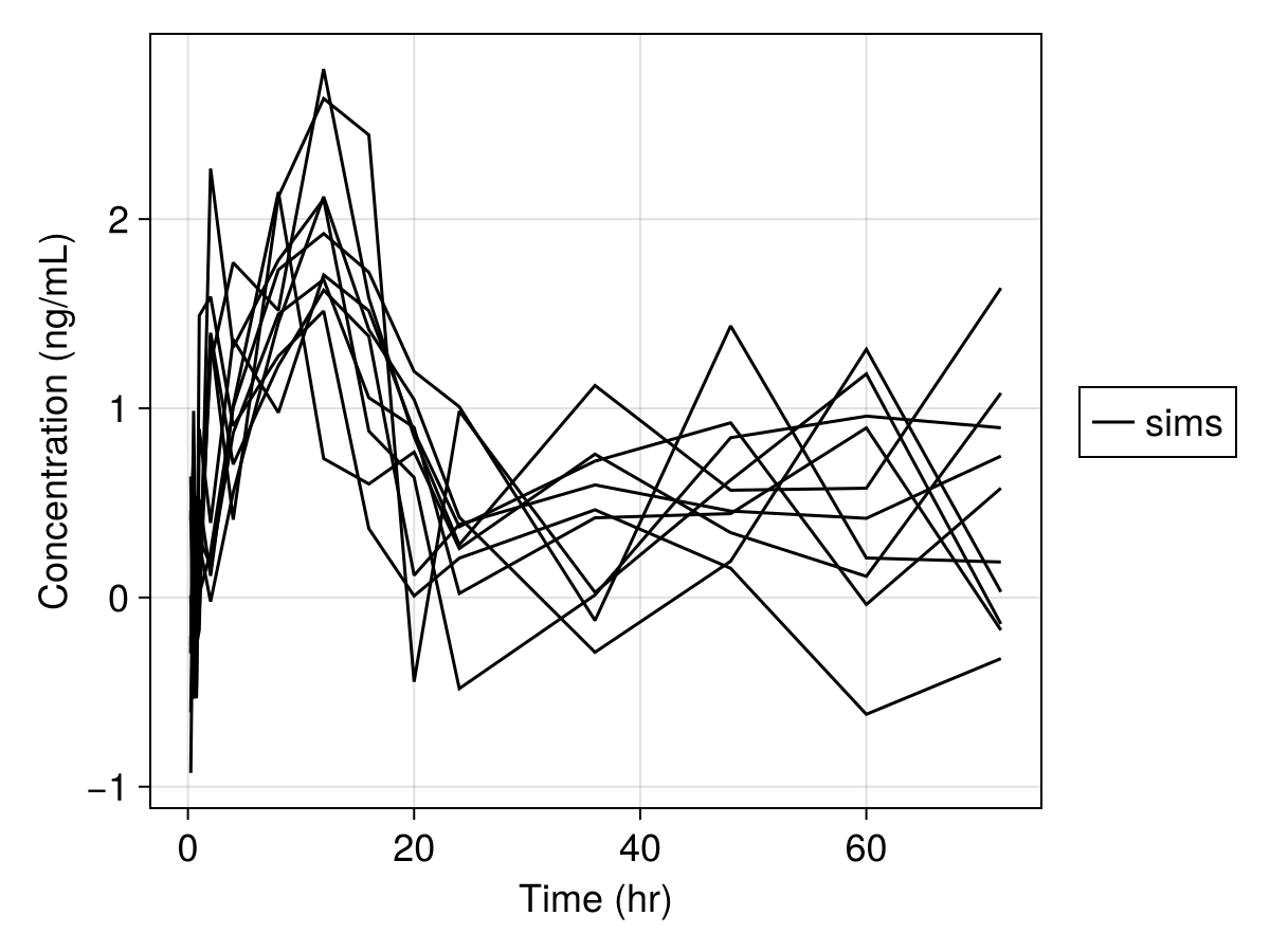
  Simulated variables: dv, resp

sim_plot(
  inf_2cmt_lin_turnover,
  sims, observations =[:dv],
  figure = (fontsize = 18, ),
  axis = (
    xlabel = "Time (hr)",
    ylabel = "Concentration (ng/mL)",
  )
)

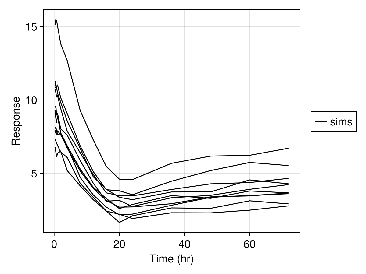
sim_plot(
  inf_2cmt_lin_turnover,
  sims, observations =[:resp],
  figure = (fontsize = 18, ),
  axis = (
    xlabel = "Time (hr)",
    ylabel = "Response",
  )
)

In this code, we defined a nonlinear mixed effects model by describing the parameters, the random effects, the dynamical model, and the derived (result) values. Then we generated a population of 10 subjects who received a single dose of 150mg, specified parameter values, simulated the model, and generated a plot of the results. Now let's walk through this process!

Using the Model Macro

First we define the model. The simplest way to do is via @model. Inside of the @model block we have a few subsections. The first of these is a @param block. In here we define what kind of parameters we have. For this model we will define structural model parameters of PK and PD and their corresponding variances where applicable:

@param begin
  tvcl ∈ RealDomain(lower = 0)
  tvvc ∈ RealDomain(lower = 0)
  tvq ∈ RealDomain(lower = 0)
  tvvp ∈ RealDomain(lower = 0)
  Ω_pk ∈ PDiagDomain(4)
  σ_prop_pk ∈ RealDomain(lower = 0)
  σ_add_pk ∈ RealDomain(lower = 0)
  # PD parameters
  tvturn ∈ RealDomain(lower = 0)
  tvebase ∈ RealDomain(lower = 0)
  tvec50 ∈ RealDomain(lower = 0)
  Ω_pd ∈ PDiagDomain(1)
  σ_add_pd ∈ RealDomain(lower = 0)
end

Next we define our random effects. The random effects are defined by a distribution from the Distributions.jl package. For more information on defining distributions, please see the Distributions.jl documentation. For this tutorial, we wish to have a multivariate normal of uncorrelated random effects, one for PK and another for PD so we utilize the syntax:

@random begin
  ηpk ~ MvNormal(Ω_pk)
  ηpd ~ MvNormal(Ω_pd)
end

Now we define our pre-processing step in @pre. This is where we choose how the parameters, random effects, and the covariates collate. We define the values and give them a name as follows:

@pre begin
  CL = tvcl * exp(ηpk[1])
  Vc = tvvc * exp(ηpk[2])
  Q = tvq * exp(ηpk[3])
  Vp = tvvp * exp(ηpk[4])

  ebase = tvebase * exp(ηpd[1])
  ec50 = tvec50
  emax = 1
  turn = tvturn
  kout = 1 / turn
  kin0 = ebase * kout
end

Next we define the @init block which gives the initial values for our differential equations. Any variable not mentioned in this block is assumed to have a zero for its starting value. We wish to only set the starting value for Resp, and thus we use:

@init begin
  Resp = ebase
end

Now we define our dynamics. We do this via the @dynamics block. Differential variables are declared by having a line defining their derivative. For our model, we use:

@dynamics begin
  Central' = -(CL / Vc) * Central + (Q / Vp) * Peripheral - (Q / Vc) * Central
  Peripheral' = (Q / Vc) * Central - (Q / Vp) * Peripheral
  Resp' = kin - kout * Resp
end

Next we setup alias variables that can be used later in the code. Such alias code can be setup in the @vars block:

@vars begin
  conc := Central / Vc
  edrug := emax * conc / (ec50 + conc)
  kin := kin0 * (1 - edrug)
end

Lastly we utilize the @derived macro to define our post-processing. We can output values using the following:

@derived begin
  dv ~ @. Normal(conc, sqrt((conc * σ_prop_pk)^2 + σ_add_pk^2))
  resp ~ @. Normal(Resp, σ_add_pd)
end

Building a Subject

Now let's build a subject to simulate the model with. A subject is defined by the following components:

1. An identifier - id
2. The dosage regimen - events
3. The covariates of the individual - covariates
4. Observations associated with the individual - observations
5. The timing of the sampling - time
6. A vector of times if the covariates are time-varying - covariate_time
7. Interpolation direction for covariates - covariate_direction

Our model did not make use of covariates so we will ignore covariate components 3, 6 and 7 for now, and observations (4) are only necessary for fitting parameters to data which will not be covered in this tutorial. Thus our subject will be defined simply by its dosage regimen.

To do this, we use the DosageRegimen constructor. The first value is always the dosing amount. Optionally, additional arguments can be specified. The most important one is time which specifies the time that the dosing occurs. For example,

DosageRegimen(150, time=0)

is a dosage regimen with a single dose of amount 150 at time t=0. Let's assume the dose is an infusion administered at the rate of 10 mg/hour into the first compartment:

regimen = DosageRegimen(150, rate=10, cmt=1)

Let's define our subject to have id=1 and this multiple dosing regimen:

subject = Subject(id = 1, events = regimen)

Subject
  ID: 1
  Events: 2

You can also create a collection of subjects as a Population.

pop = Population(map(i -> Subject(id= i, events = regimen), 1:10))

Population
  Subjects: 10
  Observations: 

Running a Simulation

The main function for running a simulation is simobs. simobs on a Population simulates all subjects of the population, while simobs on a Subject simulates just that subject. If we wish to change the parameters from the initialized values, then we pass them in. Let's simulate subject 1 with a set of chosen parameters:

turnover_params = (
  tvcl = 1.5,
  tvvc = 25.0,
  tvq = 5.0,
  tvvp = 150.0,
  tvturn = 10,
  tvebase = 10,
  tvec50 = 0.3,
  Ω_pk = Diagonal([0.05, 0.05, 0.05, 0.05]),
  Ω_pd = Diagonal([0.05]),
  σ_prop_pk = 0.15,
  σ_add_pk = 0.5,
  σ_add_pd = 0.2
)

sims = simobs(
 inf_2cmt_lin_turnover,
  pop,
  turnover_params,
  obstimes = sd_obstimes,
  rng = StableRNG(123),
)

Simulated population (Vector{<:Subject})
  Simulated subjects: 10
  Simulated variables: dv, resp

We can then plot the simulated observations by using the sim_plot command:

sim_plot(inf_2cmt_lin_turnover, sims, observations = :dv)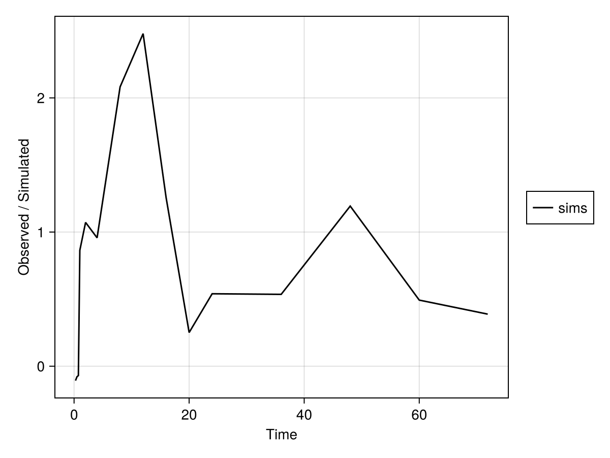

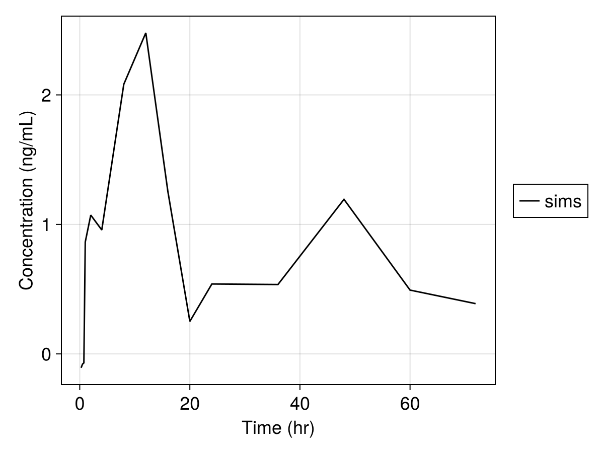
Note that we can further modify the plot, see Customizing Plots. For example,

sim_plot(
  inf_2cmt_lin_turnover,
  sims, observations =[:dv],
  figure = (fontsize = 18,),
  axis = (
    xlabel = "Time (hr)",
    ylabel = "Concentration (ng/mL)",
  )
)

When we only give the parameters, the random effects are automatically sampled from their distributions. If we wish to prescribe a value for the random effects, we pass initial values similarly:

rng = StableRNG(123)
vrandeffs = [(ηpk = rand(rng, 4), ηpd = rand(rng, 1),) for _ in pop]
sims = simobs(
  inf_2cmt_lin_turnover,
  pop,
  turnover_params,
  vrandeffs,
  obstimes = sd_obstimes,
  rng = rng,
)

Simulated population (Vector{<:Subject})
  Simulated subjects: 10
  Simulated variables: dv, resp

If a population simulation is required with the random effects set to zero, then it is possible to use the zero_randeffs function:

etas = zero_randeffs(
  inf_2cmt_lin_turnover,
  turnover_params,
  pop
)

sims = simobs(
  inf_2cmt_lin_turnover,
  pop,
  turnover_params,
  etas;
  obstimes = sd_obstimes,
  rng = StableRNG(123),
)

fig = Figure(resolution=(1000,600))

sim_plot(
  fig[1,1], inf_2cmt_lin_turnover,
  sims, observations =[:dv],
  figure = (fontsize = 18,),
  axis = (
    xlabel = "Time (hr)",
    ylabel = "Concentration (ng/mL)",
  )
)

sim_plot(
  fig[1,2], inf_2cmt_lin_turnover,
  sims, observations =[:resp],
  figure = (fontsize = 18,),
  axis = (
    xlabel = "Time (hr)",
    ylabel = "Response",
  )
)

fig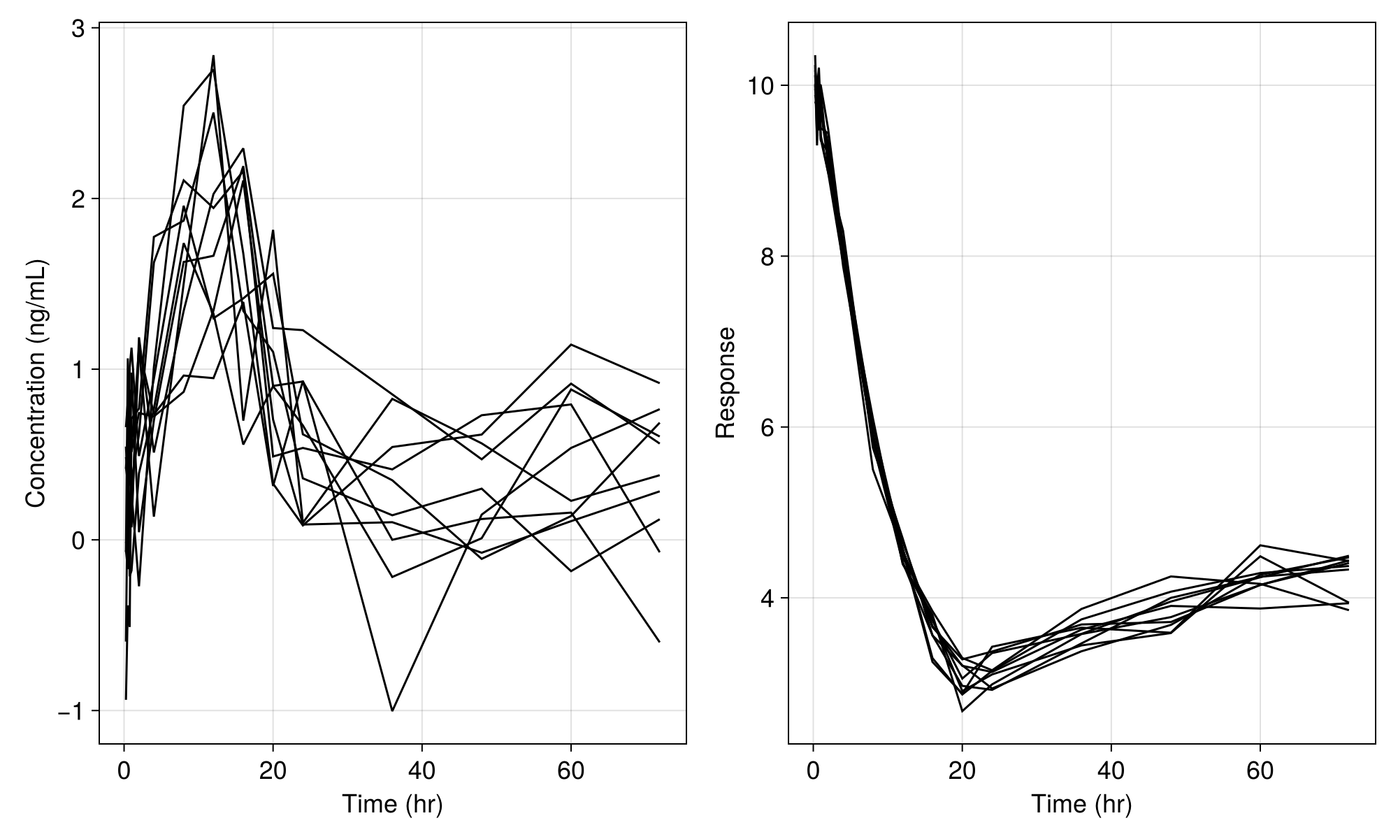

You still see variability in the plot above, mainly due to the residual variability components in the model. If we set the variance parameters to zero as below

turnover_params_wo_sigma  = (turnover_params..., σ_prop_pk = 0.0, σ_add_pk = 0.0, σ_add_pd = 0.0)

(tvcl = 1.5,
 tvvc = 25.0,
 tvq = 5.0,
 tvvp = 150.0,
 tvturn = 10,
 tvebase = 10,
 tvec50 = 0.3,
 Ω_pk = [0.05 0.0 0.0 0.0; 0.0 0.05 0.0 0.0; 0.0 0.0 0.05 0.0; 0.0 0.0 0.0 0.05],
 Ω_pd = [0.05;;],
 σ_prop_pk = 0.0,
 σ_add_pk = 0.0,
 σ_add_pd = 0.0,)

and perform the simulation without random effects again we get only the population mean:

etas = zero_randeffs(
  inf_2cmt_lin_turnover,
  turnover_params,
  pop
)

sims = simobs(
  inf_2cmt_lin_turnover,
  pop,
  turnover_params_wo_sigma,
  etas;
  obstimes = sd_obstimes,
  rng = StableRNG(123),
)

fig = Figure(resolution=(1000,600))

sim_plot(
  fig[1,1], inf_2cmt_lin_turnover,
  sims, observations =[:dv],
  figure = (fontsize = 18,),
  axis = (
    xlabel = "Time (hr)",
    ylabel = "Concentration (ng/mL)",
  )
)

sim_plot(
  fig[1,2], inf_2cmt_lin_turnover,
  sims, observations =[:resp],
  figure = (fontsize = 18, ),
  axis = (
    xlabel = "Time (hr)",
    ylabel = "Response",
  )
)

fig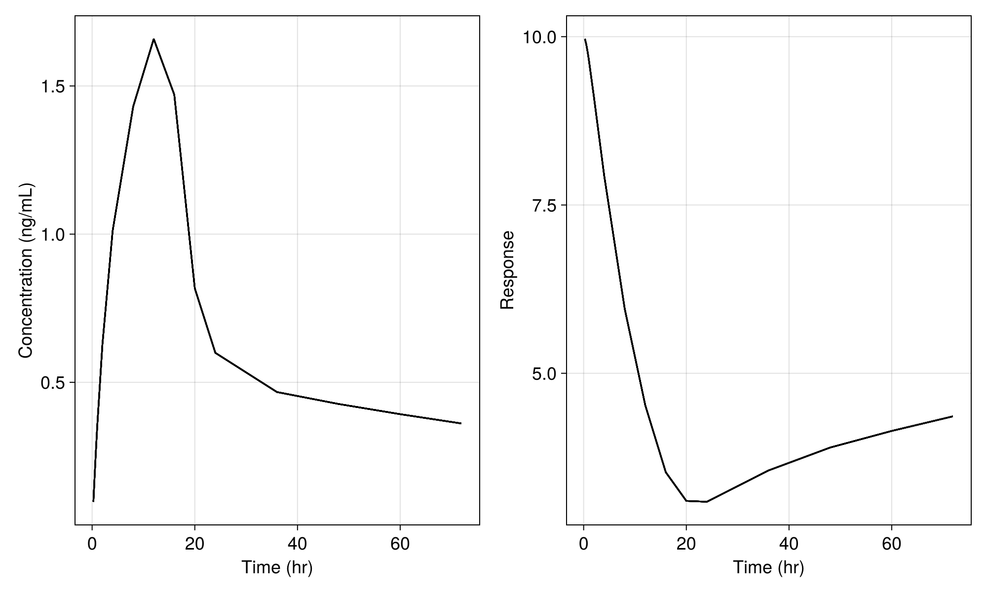

Handling the resulting SimulatedObservations

The resulting sims object contains the results of the simulation for each subject. The results for the ith subject can be retrieved by sims[i] and are of type SimulatedObservations. Each SimulatedObservations has two fields: sims[i].time is an array of time points for which the data was saved. sims[i].observations is the result of the derived variables. From there, the derived variables are accessed by name. For example,

sims[1].observations[:dv]

is the array of dv values at the associated time points for subject 1. We can convert the simulation results to Pumas Subjects using the constructor broadcasted over all elements of sims:

sims_subjects = Subject.(sims)

Population
  Subjects: 10
  Observations: dv, resp

Then sims_subjects can be used to fit the model parameters based on the simulated dataset. We can also turn the simulated population into a DataFrame with the DataFrame constructor:

DataFrame(sims)

From there, any Julia tools can be used to analyze these arrays and DataFrames.

Conducting an Estimation

With a model and population you can fit your model. Model fitting in Pumas has the purpose of estimate parameters and is done by calling the fit function with the following positional arguments:

1. a Pumas model.
2. a Population or a Subject.
3. a named tuple of the initial parameter values.
4. an inference algorithm.

If you want to use the model's initial parameter values declared inside the @param block, you can do so with init_params(model). Note that this will fall back to the parameters' default values if you do not specify an initial value inside the @param block.

Pumas supports the following inference algorithms:

• Maximum Likelihood Estimation:
  • NaivePooled(): first order approximation without random-effects.
  • FO(): first-order approximation.
  • FOCE(): first-order conditional estimation.
  • LaplaceI(): second-order Laplace approximation.
  • SAEM: Stochastic Approximation using the Expectation-Maximization algorithm. Note that you need an @emmodel instead of a @model.
• Bayesian inference:
  • BayesMCMC(): MCMC using No-U-Turn Sampler (NUTS).
  • MAP(): Maximum A Posteriori estimation.

Now we can fit our model using one of the simulated populations from the previous section:

turnover_params = (
  tvcl = 1.5,
  tvvc = 25.0,
  tvq = 5.0,
  tvvp = 150.0,
  tvturn = 10,
  tvebase = 10,
  tvec50 = 0.3,
  Ω_pk = Diagonal([0.05, 0.05, 0.05, 0.05]),
  Ω_pd = Diagonal([0.05]),
  σ_prop_pk = 0.15,
  σ_add_pk = 0.5,
  σ_add_pd = 0.2
)

sims = simobs(
  inf_2cmt_lin_turnover,
  pop,
  turnover_params,
  obstimes = sd_obstimes,
  rng = StableRNG(123)
)

Simulated population (Vector{<:Subject})
  Simulated subjects: 10
  Simulated variables: dv, resp

fit_2cmt_lin_turnover = fit(
  inf_2cmt_lin_turnover,
  Subject.(sims),
  init_params(inf_2cmt_lin_turnover),
  Pumas.FOCE()
)

FittedPumasModel

Successful minimization:                      true

Likelihood approximation:               Pumas.FOCE
Log-likelihood value:                   -136.79299
Number of subjects:                             10
Number of parameters:         Fixed      Optimized
                                  0             15
Observation records:         Active        Missing
    dv:                         150              0
    resp:                       150              0
    Total:                      300              0

------------------------
              Estimate
------------------------
tvcl           1.6271
tvvc          20.756
tvq            4.0536
tvvp         109.18
Ω_pk₁,₁        0.041114
Ω_pk₂,₂        0.091621
Ω_pk₃,₃        0.0362
Ω_pk₄,₄        0.027386
σ_prop_pk      0.070826
σ_add_pk       0.46577
tvturn         9.9485
tvebase       11.123
tvec50         0.32579
Ω_pd₁,₁        0.069718
σ_add_pd       0.2002
------------------------

Calculating confidence intervals and Bootstrap

You can calculate confidence intervals using the infer function (by default 95% CIs):

infer_2cmt_lin_turnover = infer(fit_2cmt_lin_turnover)

Asymptotic inference results using sandwich estimator

Successful minimization:                      true

Likelihood approximation:               Pumas.FOCE
Log-likelihood value:                   -136.79299
Number of subjects:                             10
Number of parameters:         Fixed      Optimized
                                  0             15
Observation records:         Active        Missing
    dv:                         150              0
    resp:                       150              0
    Total:                      300              0

----------------------------------------------------------------------
             Estimate          SE                     95.0% C.I.
----------------------------------------------------------------------
tvcl          1.6271         0.21575         [ 1.2042   ;   2.0499  ]
tvvc         20.756          2.3862          [16.079    ;  25.433   ]
tvq           4.0536         0.37332         [ 3.322    ;   4.7853  ]
tvvp        109.18          10.902           [87.809    ; 130.55    ]
Ω_pk₁,₁       0.041114       0.023954        [-0.0058346;   0.088062]
Ω_pk₂,₂       0.091621       0.048107        [-0.0026665;   0.18591 ]
Ω_pk₃,₃       0.0362         0.032671        [-0.027834 ;   0.10023 ]
Ω_pk₄,₄       0.027386       0.025893        [-0.023362 ;   0.078135]
σ_prop_pk     0.070826       0.17202         [-0.26633  ;   0.40798 ]
σ_add_pk      0.46577        0.045772        [ 0.37606  ;   0.55548 ]
tvturn        9.9485         0.38629         [ 9.1914   ;  10.706   ]
tvebase      11.123          0.93216         [ 9.2961   ;  12.95    ]
tvec50        0.32579        0.027227        [ 0.27243  ;   0.37916 ]
Ω_pd₁,₁       0.069718       0.01392         [ 0.042436 ;   0.097001]
σ_add_pd      0.2002         0.014756        [ 0.17127  ;   0.22912 ]
----------------------------------------------------------------------

You can also convert the output to a DataFrame with the coeftable function:

coeftable(infer_2cmt_lin_turnover)

For inference with bootstrap-based confidence intervals you can use Pumas.Bootstrap as an optional second positional argument in infer (by default the number of samples is 200):

infer_boot_2cmt_lin_turnover = infer(fit_2cmt_lin_turnover, Pumas.Bootstrap(ensemblealg=EnsembleThreads()))

┌ Info: Bootstrap inference finished.
│   Total resampled fits = 200
│   Success rate = 1.0
└   Unique resampled populations = 200
Bootstrap inference results

Successful minimization:                      true

Likelihood approximation:               Pumas.FOCE
Log-likelihood value:                   -144.42225
Number of subjects:                             10
Number of parameters:         Fixed      Optimized
                                  0             15
Observation records:         Active        Missing
    dv:                         150              0
    resp:                       150              0
    Total:                      300              0

----------------------------------------------------------------------
             Estimate          SE                     95.0% C.I.
----------------------------------------------------------------------
tvcl          1.1668         0.30297       [  0.55865   ;   1.5918  ]
tvvc         23.26           4.1501        [ 18.107     ;  32.552   ]
tvq           5.1594         0.49696       [  4.3548    ;   6.2169  ]
tvvp        171.12          49.577         [119.58      ; 308.94    ]
Ω_pk₁,₁       0.038306       1.599         [  2.2387e-16;   0.10429 ]
Ω_pk₂,₂       0.086399       0.044714      [  1.1596e-9 ;   0.17843 ]
Ω_pk₃,₃       0.023877       0.012185      [  5.6738e-18;   0.043998]
Ω_pk₄,₄       0.093753       0.044657      [  0.010312  ;   0.17991 ]
σ_prop_pk     0.076458       0.076803      [  1.9102e-10;   0.21935 ]
σ_add_pk      0.51079        0.03356       [  0.4362    ;   0.55698 ]
tvturn       10.221          0.59544       [  9.016     ;  11.213   ]
tvebase       9.5673         0.64726       [  8.3718    ;  10.83    ]
tvec50        0.30015        0.037184      [  0.23985   ;   0.38186 ]
Ω_pd₁,₁       0.047302       0.013862      [  0.016567  ;   0.069705]
σ_add_pd      0.20055        0.011621      [  0.17741   ;   0.2248  ]
----------------------------------------------------------------------
Successful fits: 200 out of 200
Unique resampled populations: 200
No stratification.

You can also convert the inference results to a DataFrame with coeftable:

coeftable(infer_boot_2cmt_lin_turnover)

julia> coeftable(infer_boot_2cmt_lin_turnover)
15×5 DataFrame
 Row │ parameter  estimate     se          ci_lower       ci_upper
     │ String     Float64      Float64     Float64        Float64
─────┼────────────────────────────────────────────────────────────────
   1 │ tvcl         1.16678     0.302968     0.558649       1.59179
   2 │ tvvc        23.2605      4.15007     18.1071        32.5522
   3 │ tvq          5.15943     0.496956     4.35485        6.21692
   4 │ tvvp       171.116      49.5771     119.585        308.94
   5 │ Ω_pk₁,₁      0.0383064   1.59895      2.2387e-16     0.10429
   6 │ Ω_pk₂,₂      0.0863987   0.0447138    1.15956e-9     0.178432
   7 │ Ω_pk₃,₃      0.0238772   0.0121848    5.67381e-18    0.0439976
   8 │ Ω_pk₄,₄      0.093753    0.0446573    0.0103117      0.179912
   9 │ σ_prop_pk    0.0764577   0.0768028    1.9102e-10     0.219353
  10 │ σ_add_pk     0.510786    0.0335596    0.436204       0.556977
  11 │ tvturn      10.2212      0.595444     9.01602       11.2135
  12 │ tvebase      9.56727     0.647258     8.37178       10.8296
  13 │ tvec50       0.300155    0.0371844    0.239847       0.381857
  14 │ Ω_pd₁,₁      0.0473021   0.0138622    0.0165671      0.0697046
  15 │ σ_add_pd     0.200548    0.011621     0.177408       0.224798

Conclusion

This tutorial covered the basic workflow of building a model, simulating results from it, and conducting an estimation. The subsequent tutorials will discuss the components in more detail, such as:

1. More detailed treatment of specifying populations, dosage regimens, and covariates.
2. Reading in dosage regimens and observations from standard input data.
3. Fitting models with different estimation methods.