Non-Compartmental Analysis (NCA) in Pumas
The NCA analysis itself is documented in the NCA.jl section of this manual: Data Parsing for reading the data, Running NCA for computing and summarizing the endpoints, and Endpoint Reference for the endpoints themselves.
This page covers what surrounds it in Pumas: getting the source data in, plotting the data and the results, and running NCA on a simulation of a Pumas model instead of on a dataset.
Read Source Data
Data Parsing provides the specification requirements of the source data. Currently, several file formats can be read in for analysis:
.csv(CSVpackage).xlsx(XLSXpackage).sas7bdat/.xpt(ReadStatTablespackage).arrow(Arrowpackage)
For this introduction we'll use the PharmaDatasets package and the po_sad_1 dataset:
using PharmaDatasets

pkdata = dataset("po_sad_1")
first(pkdata, 6)| Row | id | time | dv | amt | evid | cmt | rate | age | wt | doselevel | isPM | isfed | sex | route |
|---|---|---|---|---|---|---|---|---|---|---|---|---|---|---|
| Int64 | Float64 | Float64? | Float64? | Int64 | Int64? | Float64 | Int64 | Int64 | Int64 | String3 | String3 | String7 | String3 | |
| 1 | 1 | 0.0 | missing | 30.0 | 1 | 1 | 0.0 | 51 | 74 | 30 | no | yes | male | ev |
| 2 | 1 | 0.25 | 35.7636 | missing | 0 | missing | 0.0 | 51 | 74 | 30 | no | yes | male | ev |
| 3 | 1 | 0.5 | 71.9551 | missing | 0 | missing | 0.0 | 51 | 74 | 30 | no | yes | male | ev |
| 4 | 1 | 0.75 | 97.3356 | missing | 0 | missing | 0.0 | 51 | 74 | 30 | no | yes | male | ev |
| 5 | 1 | 1.0 | 128.919 | missing | 0 | missing | 0.0 | 51 | 74 | 30 | no | yes | male | ev |
| 6 | 1 | 2.0 | 155.85 | missing | 0 | missing | 0.0 | 51 | 74 | 30 | no | yes | male | ev |
In po_sad_1 the dosing events are interleaved with the observations: a dose is its own row, carrying the amount in amt, and the observation rows leave amt empty. That layout is read with read_nca_pumas:
using NCA

ncadata = read_nca_pumas(pkdata; concentration = :dv, dose = :amt, group = [:doselevel])
first(ncadata, 6)| Row | doselevel | id | profile | time | nominal_time | dose_time | nominal_dose_time | concentration | dose | route | duration | exclusion | exclusion_mask |
|---|---|---|---|---|---|---|---|---|---|---|---|---|---|
| Int64 | Int64 | Int64 | Float64 | Float64 | Float64 | Float64 | Float64 | Float64 | String | Missing | Missing | Bool | |
| 1 | 30 | 1 | 1 | 0.25 | 0.25 | 0.0 | 0.0 | 35.7636 | 30.0 | ev | missing | missing | false |
| 2 | 30 | 1 | 1 | 0.5 | 0.5 | 0.0 | 0.0 | 71.9551 | 30.0 | ev | missing | missing | false |
| 3 | 30 | 1 | 1 | 0.75 | 0.75 | 0.0 | 0.0 | 97.3356 | 30.0 | ev | missing | missing | false |
| 4 | 30 | 1 | 1 | 1.0 | 1.0 | 0.0 | 0.0 | 128.919 | 30.0 | ev | missing | missing | false |
| 5 | 30 | 1 | 1 | 2.0 | 2.0 | 0.0 | 0.0 | 155.85 | 30.0 | ev | missing | missing | false |
| 6 | 30 | 1 | 1 | 4.0 | 4.0 | 0.0 | 0.0 | 191.835 | 30.0 | ev | missing | missing | false |
Exploratory Data Analysis
Exploratory analysis of the profiles can be performed using the plotting functions that come with NCA. The NCA plots section provides more details, but here are some example syntax and the corresponding plots.
Observations-time plots
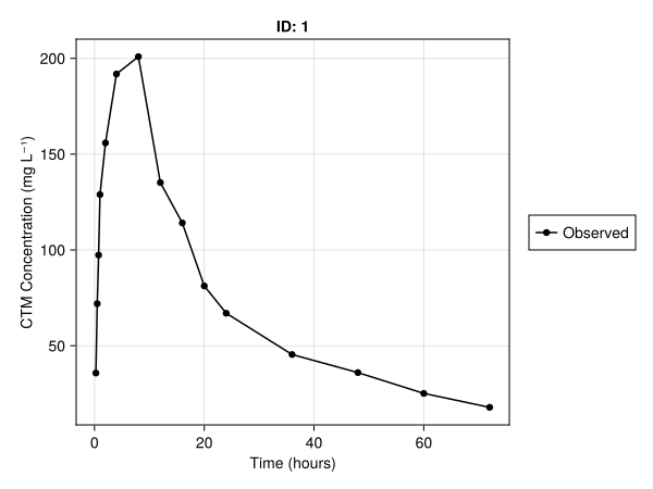
We can produce a plot of the concentration against time using observations_vs_time. Below is the code for generating this plot for the first subject, selected with the usual DataFrame filtering:
using DataFrames

subject1 = filter(:id => ==(1), ncadata)
observations_vs_time(
    subject1;
    axis = (; xlabel = "Time (hours)", ylabel = "CTM Concentration (mg L⁻¹)"),
)
We can also use log-scale for the concentrations such that exponential decay shows as a straight line. Below is the code to set the y-scale to use the natural logarithm:
observations_vs_time(
    subject1;
    axis = (; xlabel = "Time (hours)", ylabel = "CTM Concentration (mg L⁻¹)", yscale = log),
)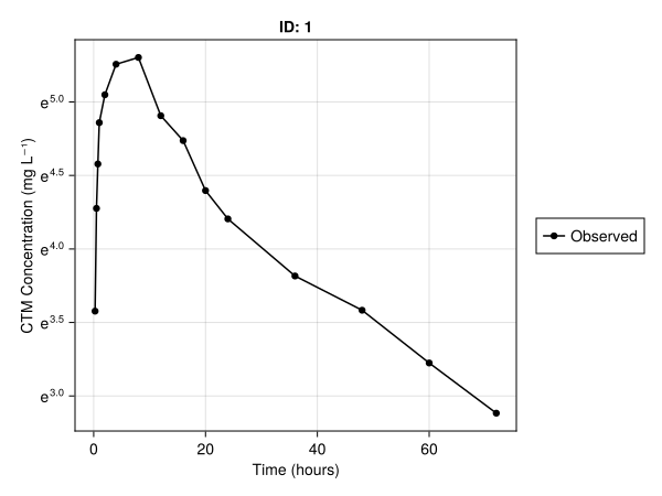
Other options are yscale = log10 and yscale = log2 for a base-10 and base-2 logarithm.
To generate these plots side-by-side we have to create a Figure-object first, and then pass fig[row,column] as the first argument. row specifies which row of the figure the element should be added to and column specifies the column number.
using CairoMakie
fig = Figure()
observations_vs_time(
    fig[1, 1],
    subject1;
    axis = (; xlabel = "Time (hours)", ylabel = "CTM Concentration (mg L⁻¹)"),
)
observations_vs_time(
    fig[1, 2],
    subject1;
    axis = (; xlabel = "Time (hours)", ylabel = "CTM Concentration (mg L⁻¹)", yscale = log),
)
fig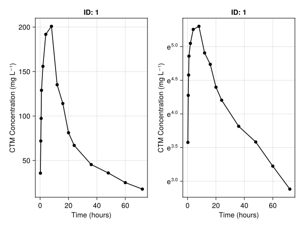
Summary plots
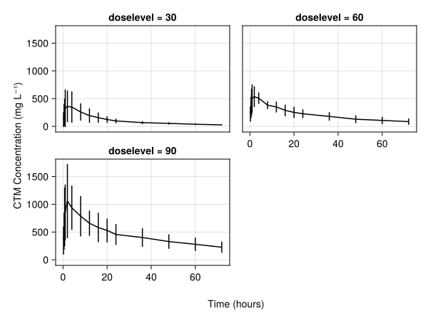
We can also group all the subjects into a single summarizing plot of the concentration against time using summary_observations_vs_time:
summary_observations_vs_time(
    ncadata;
    axis = (; xlabel = "Time (hours)", ylabel = "CTM Concentration (mg L⁻¹)"),
)
Subject fit plots
We can also check all the subject fits with:
subject_fits(ncadata; axis = (; yscale = log), rows = 3, columns = 3)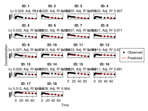
Plot the results
The endpoints are computed with run_nca, described in Running NCA:
pk_nca = run_nca(ncadata)Several of the plotting functions take that result rather than the profiles.
Parameter distributions
parameters_dist(pk_nca; parameter = :aucinf_obs, rows = 3, columns = 1)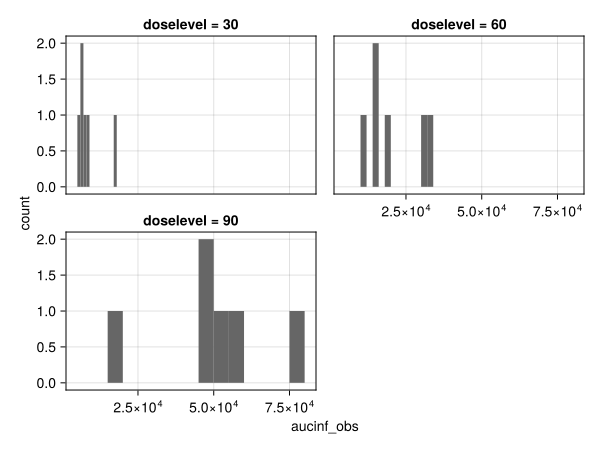
Parameter distribution by groups (ID or covariates)
parameters_vs_group(pk_nca; parameter = :aucinf_obs)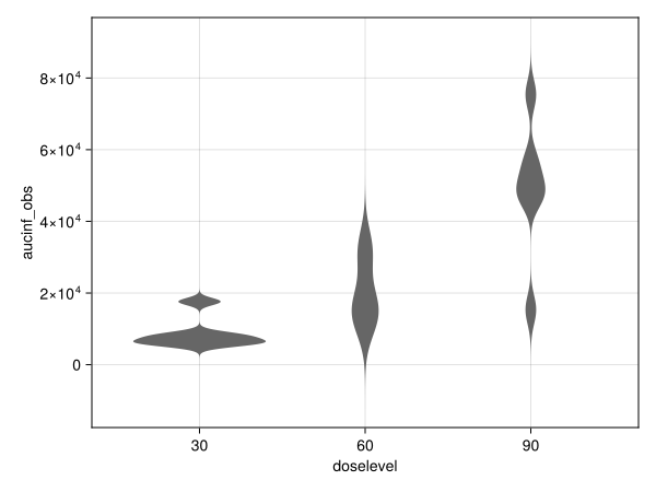
Dose linearity
DoseLinearityPowerModel fits a power regression model between dose and one of the endpoints, and power_model visualizes it:
dose_lin = DoseLinearityPowerModel(pk_nca, :aucinf_obs; level = 0.95)
power_model(dose_lin)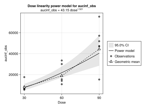
NCA on a simulation of a model
Pumas also provides a convenient way to perform NCA on the output of a simulation of a Pumas model, rather than on a dataset. This is discussed in the Model integrated NCA section.