Visual Predictive Check (VPC)
Pumas allows you to generate VPC quantiles for your data and model simulations and utilize the Julia plotting capabilities to generate the relevant VPC plots. This is allowed with the vpc function.
VPC with Simulation
Pumas.vpc — Method
vpc(
  fpm::AbstractFittedPumasModel;
  samples::Integer = 499
  qreg_method = IP(),
  observations::Vector{Symbol} = [keys(fpm.data[1].observations)[1]],
  stratify_by::Vector{Symbol} = Symbol[],
  quantiles::NTuple{3,Float64}=(0.1, 0.5, 0.9),
  level::Real=0.95,
  ensemblealg=EnsembleThreads(),
  bandwidth=nothing,
  maxnumstrats=[6 for i in 1:length(stratify_by)],
  covariates::Vector{Symbol} = [:time],
  smooth::Bool = true,
  rng::AbstractRNG=default_rng(),
  nodes::Dict = Dict{Tuple{},Vector{Float64}}(),
  nnodes::Integer = 0,
  prediction_correction = false,
)
Compute the quantiles for VPC for a FittedPumasModel or FittedPumasEMModel with simulated confidence intervals around the empirical quantiles based on samples simulated populations.
The following keyword arguments are supported:
samples: The number of simulated populations to generate, defaults to499quantiles::NTuple{3,Float64}: A three-tuple of the quantiles for which the quantiles will be computed. The default is(0.1, 0.5, 0.9)which computes the 10th, 50th and 90th percentile.level::Real: Probability level to use for the simulated confidence intervals. The default is0.95.observations::Vector{Symbol}: The name of the dependent variable to use for the VPCs. The default is the first dependent variable in thePopulation.stratify_by: The covariates to be used for stratification. Takes anVectorof theSymbols of the stratification covariates.ensemblealg: This is the parallelization choice.bandwidth: The kernel bandwidth in the quantile regression. If you are seeingNaNs or an error, increasing the bandwidth should help in most cases. With higher values of thebandwidthyou will get more smoothened plots of the quantiles so it's a good idea to check with your data to pick the rightbandwidth. For a ContinuousVPC, the default value is 2.0. For a DiscreteVPC, the default value is nothing to indicate automatic bandwidth tuning. For a CensoredVPC, the bandwidth should be given as a tuple where the first value applies to the ContinuousVPC and the second to the DiscreteVPC for the censoring variable. For example,(4.0, nothing)applies a bandwidth of4.0to the ContinuousVPC and automatically tunes the DiscreteVPC. Automatic tuning is only applicable to DiscreteVPCs at this moment.maxnumstrats: The maximum number of strata for each covariate. Takes an Vector with the number of strata for the corresponding covariate, passed instratify_by. It defaults to6for each of the covariates.covariates: The independent variable for VPC, defaults to[:time].smooth: In case of discrete VPC used to determine whether to interpolate the dependent variable if independent variable is continuous, defaults totrue.rng: A random number generator, uses thedefault_rngfromRandomas default.nodes: A Dict specifying the local regression nodes. Ifstratify_byargument has been specified, the dict should have tuples of values as keys corresponding to each stratum. Otherwise, the key should be an empty tuple. The values of the Dict should be the nodes of the local regressions. If thenodesargument is not passed, at mostnnodesquantiles is used from each stratum.nnodes: An integer specifying the number of points to use for the local regressions for each stratum. The default value is 11 but the actual number of nodes will not exceed the number of unique covariate values in the stratum.qreg_method: Defaults toIP(). For most users the method used in quantile regression is not going to be of concern, but if you see large run times switchingqreg_methodtoIP(true)should help in improving the performance with a tradeoff in the accuracy of the fitting.prediction_correction: Default tofalse. Set totrueto enable prediction correction that multiplies all observations with the ratio between the mean prediction and each individuals population prediction.
Computes the quantiles for VPC for a FittedPumasModel or FittedPumasEMModel with simulated confidence intervals around the empirical quantiles based on samples simulated populations to be input as a keyword with a default value of 499. The resulting object can then be passed to the vpc_plot function to generate the plots.
Hence, a vpc call with 100 repetitions of simulation would be:
res = fit(model, data, param, FOCE())
vpc_fpm = vpc(res; samples = 100)
The sample simulations are performed in parallel by default using multithreading (ensemblealg = EnsembleThreads()). Stratified resampling of the populations for the bootstrap fits based on the wt covariate is performed as follows:
vpc_fpm_stratwt = vpc(res; stratify_by = [:wt])
# run only 100 simulations
vpc_fpm_stratispm = vpc(res; samples = 100, stratify_by = [:isPM])
Prediction correction can be turned on by specifying prediction_correction = true
vpc_fpm = vpc(res; samples = 100, prediction_correction = true)The VPC object obtained as the result contains the following fields:
simulated_quantiles::DataFrame:DataFrameof the simulated quantiles result.popvpc::PopVPC: APopVPCobject with the observation quantiles (data_quantiles), data (data), stratification covariate if specified (stratify_by) and the dependent variable (dv).level::Float64: The simulation CI'slevel.
Since the quantiles are stored as DataFrames it is very easy to use the result of vpc and also export it using CSV package to your disk.
vpc_fpm.simulated_quantiles
vpc_fpm.popvpc.data_quantiles

using CSV
CSV.write("sim_quantiles.csv", vpc_fpm.simulated_quantiles)
In Pumas, for models with continuous derived variables (including prediction corrected VPCs), the non-parametric quantile regression approach discussed in Jamsen et al. is used. Discrete and Time to Event models are also supported through the vpc function and can be used without any change in syntax.
Full examples
Let's take a look at a complete example, first we define the model and generate round-trip data.
using Pumas
using PumasUtilities
using DataFrames
using LinearAlgebra
model = @model begin
@param begin
tvcl ∈ RealDomain(; lower = 0)
tvv ∈ RealDomain(; lower = 0)
pmoncl ∈ RealDomain(; lower = -0.99)
Ω ∈ PDiagDomain(2)
σ_prop ∈ RealDomain(; lower = 0)
end
@random begin
η ~ MvNormal(Ω)
end
@covariates wt isPM
@pre begin
CL = tvcl * (1 + pmoncl * isPM) * (wt / 70)^0.75 * exp(η[1])
Vc = tvv * (wt / 70) * exp(η[2])
end
@dynamics Central1
@derived begin
cp = @. 1_000 * (Central / Vc)
dv ~ @. ProportionalNormal(cp, σ_prop)
end
end
ev = DosageRegimen(100; time = 0, addl = 2, ii = 24)
s1 = Subject(; id = 1, events = ev, covariates = (isPM = 1, wt = 70))
param = (; tvcl = 4.0, tvv = 70, pmoncl = -0.7, Ω = Diagonal([0.09, 0.09]), σ_prop = 0.04)
choose_covariates() = (; isPM = rand([1, 0]), wt = rand(55:80))
pop_with_covariates =
map(i -> Subject(; id = i, events = ev, covariates = choose_covariates()), 1:10)
obs = simobs(model, pop_with_covariates, param; obstimes = 0:1:60)
simdf = DataFrame(obs);
data = read_pumas(simdf; time = :time, covariates = [:isPM, :wt])
res = fit(model, data, param, FOCE())FittedPumasModel
Dynamical system type: Closed form
Number of subjects: 10
Observation records: Active Missing
dv: 610 0
Total: 610 0
Number of parameters: Constant Optimized
0 6
Likelihood approximation: FOCE
Likelihood optimizer: BFGS
Termination Reason: GradientNorm
Log-likelihood value: -3289.9458
------------------
Estimate
------------------
tvcl 4.1362
tvv 81.733
pmoncl -0.70569
Ω₁,₁ 0.11397
Ω₂,₂ 0.191
σ_prop 0.03992
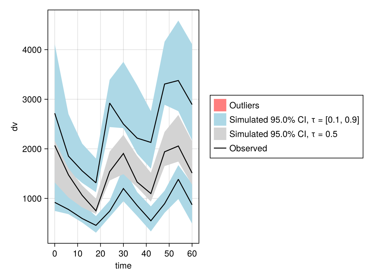
------------------vpc_fpm = vpc(res);
vpc_plot(vpc_fpm)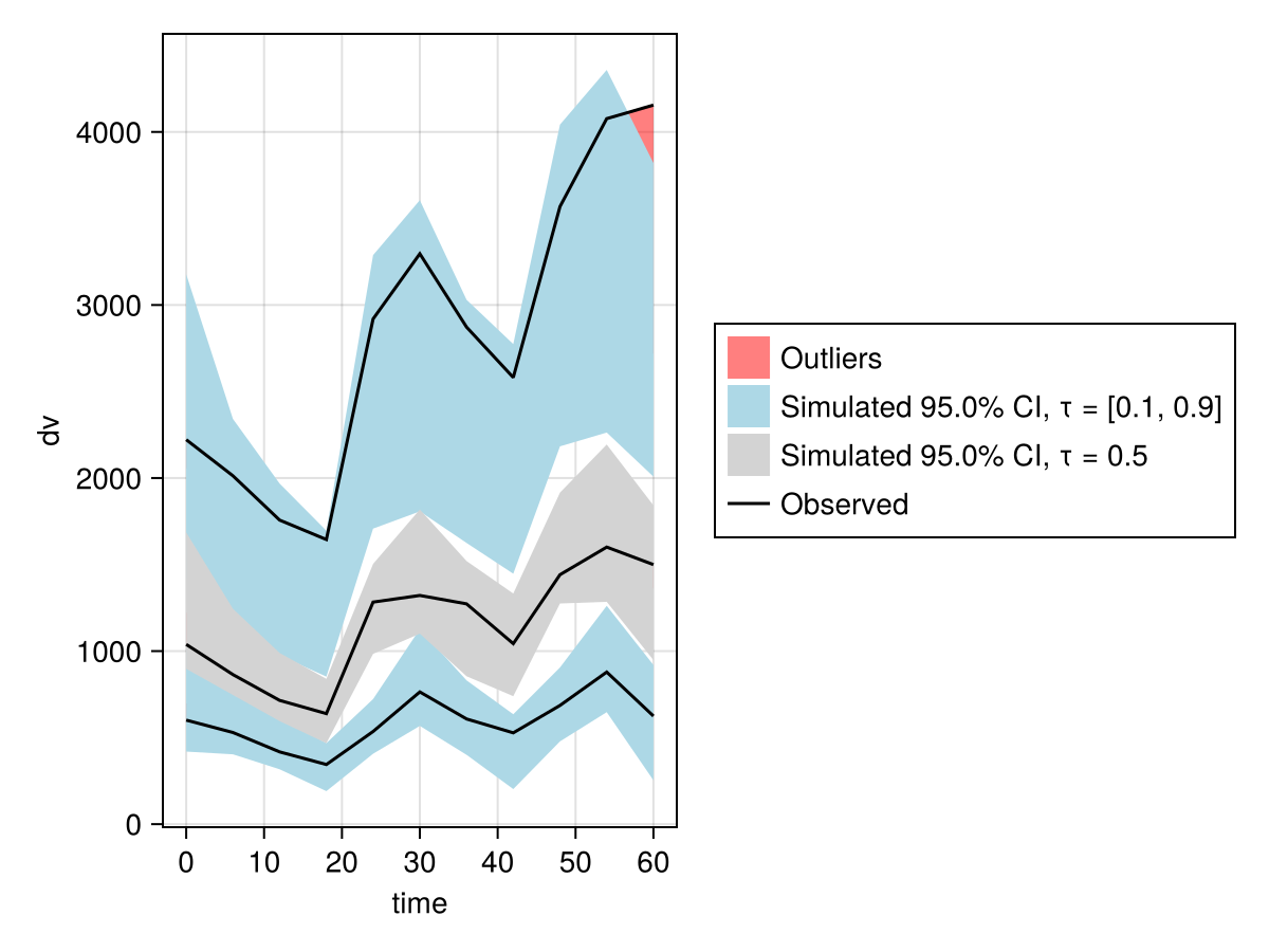
vpc_plot supports many customization options. For instance, you could change the axis limits through the axis keyword argument and the limits option:
vpc_plot(vpc_fpm; axis = (; limits = (0, 24, nothing, nothing)))In this example, we changed the limits on the x-axis to only show the first 24 hours and allowed for automatic y-axis limits by setting them to nothing.
You can find more information on how to customize plots using axis and other customization options in Pumas plots in our plotting in Julia and plot customization tutorials. Also, make sure to check the list of supported style keywords for vpc_plot and our documentation section on Customizing Plots.
Alternatively, using a PumasEMModel:
emmodel = @emmodel begin
    @random begin
        CLdw ~ 1 + isPM | LogNormal # CLdw = μ_CL * exp(μ_CL_isPM * isPM) * exp(η_CL)
        Vcdw ~ 1 | LogNormal # Vcdw = μ_Vc * exp(η_Vc)
    end
    @covariates wt
    @pre begin
        CL = CLdw * (wt / 70)^0.75
        Vc = Vcdw * (wt / 70)
    end
    @dynamics Central1
    @post begin
        cp = 1000 * Central / Vc
    end
    @error begin
        dv ~ ProportionalNormal(cp)
    end
end

emparam = (;
    CLdw = (4.0, -1.2), # -1.2 ≈ log(1 - 0.7) = log(1 - pmoncl)
    Vcdw = 70,
    Ω = (0.09, 0.09),
    σ = (0.04,),
)

emres = fit(emmodel, data, emparam, LaplaceI())

vpc_emfpm = vpc(emres);
Visual Predictive Check
Type of VPC: Continuous VPC
Simulated populations: 499
Subjects in data: 10
Stratification variable(s): None
Confidence level: 0.95
VPC lines: quantiles ([0.1, 0.5, 0.9])Note that because isPM equals either 0 or 1, pmoncl = exp(μ_CL_isPM) - 1, allowing us to perform a change of variables and express the earlier PumasModel as a PumasEMModel.
In PumasModels and PumasEMModels, you can increase performance by preprocessing covariates. Instead of wt, you can try storing (wt/70) and (wt/70)^0.75 as appropriately named covariates.
vpc_plot(vpc_emfpm)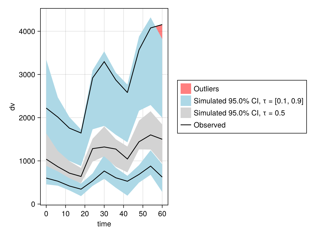
Let's generate a VPC stratified on isPM covariate with stratify_by. Note that multiple covariates can be passed to stratify_by to get cross stratified VPC plots, in that case the maxnumstrats will have to be adjusted accordingly.
resem_saem = fit(emmodel, data, (; CLdw = (5.0, 0.0), Vcdw = 50.0), SAEM())

vpc_fpmem_saem = vpc(resem_saem; samples = 100);
vpc_plot(vpc_fpmem_saem)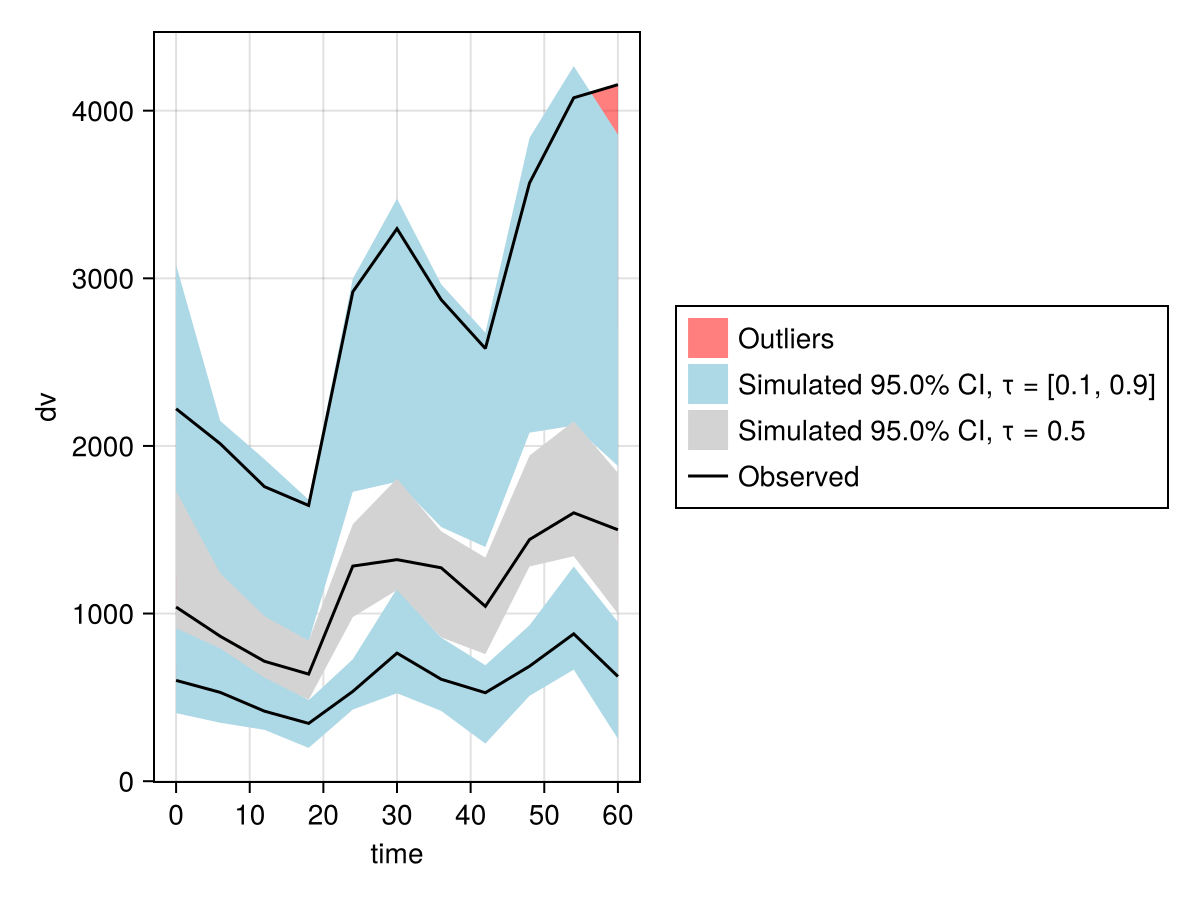
When fitting with SAEM, it is strongly recommended to use values for the Ω parameters much larger than your estimates of the true values, or to avoid providing them so they default to 1.0 along the diagonal. Using small values such as emparams will result in convergence failure.
vpc_fpm = vpc(res; stratify_by = [:isPM])
vpc_plot(vpc_fpm)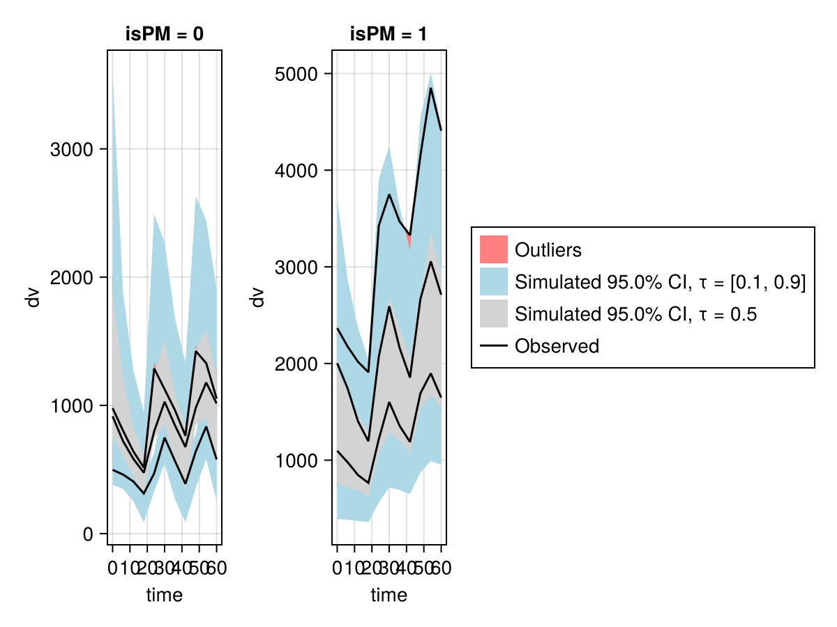
vpc_saem_fpm = vpc(resem_saem; stratify_by = [:isPM]);
vpc_plot(vpc_saem_fpm)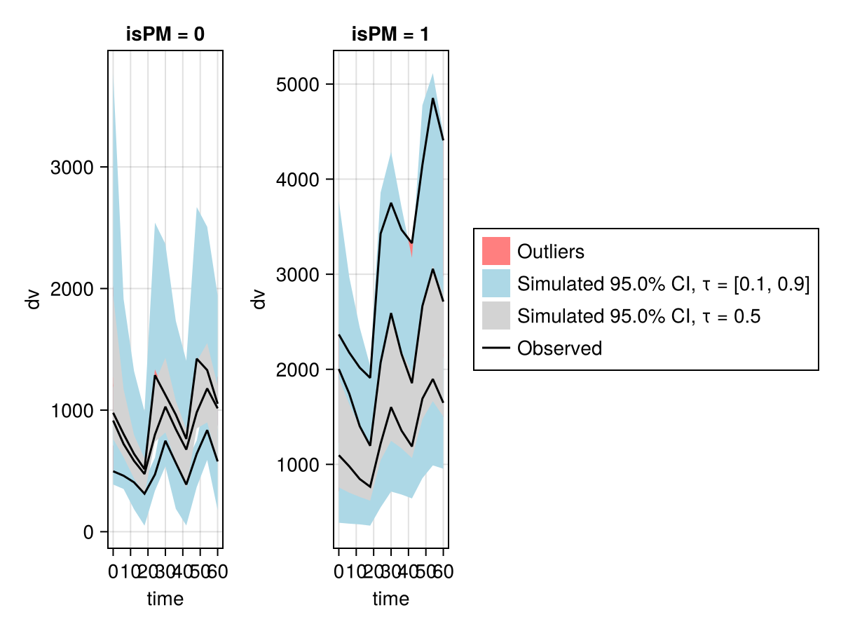
By specifying the plot and the path the VPC plot can be saved to the disk as below:
p = vpc_plot(vpc_fpm);
CairoMakie.save("obstimesvpc.png", p)
More examples of VPC plots can be found in the plotting page's vpc_plot section.
If your vpc run gives you an error message similar to ERROR: LinearAlgebra.LAPACKException(2), increasing the bandwidth should fix it in most cases.
For most users, the method used in quantile regression is not going to be of concern, but if you see large run times switching qreg_method to IP(true) after loading QuantileRegressions package should help in improving the performance with a tradeoff in the accuracy of the regression fitting.
Prediction corrected VPCs (pcVPCs) can be done with prediction_correction = true:
vpc_fpm = vpc(res; samples = 100, prediction_correction = true);
vpc_plot(vpc_fpm)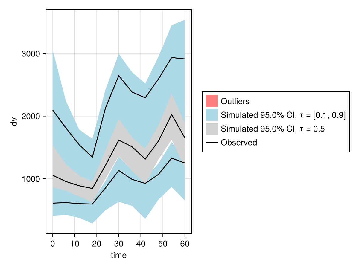
VPC after Simulation
It is also possible to run the VPC as a post-processing step on arbitrary simulation output sims from any simobs function call. For more on simulations and how to use simobs, check the Simulation of Pumas Models section of the documentation.
Example
The following is an example of simulating from a bootstrap result and then plotting a VPC using the simulations.
model = @model begin
    @param begin
        tvcl ∈ RealDomain(; lower = 0)
        tvv ∈ RealDomain(; lower = 0)
        pmoncl ∈ RealDomain(; lower = -0.99)
        Ω ∈ PDiagDomain(2)
        σ_prop ∈ RealDomain(; lower = 0)
    end

    @random begin
        η ~ MvNormal(Ω)
    end

    @covariates wt isPM

    @pre begin
        CL = tvcl * (1 + pmoncl * isPM) * (wt / 70)^0.75 * exp(η[1])
        Vc = tvv * (wt / 70) * exp(η[2])
    end

    @dynamics Central1

    @derived begin
        cp = @. 1000 * (Central / Vc)
        dv ~ @. ProportionalNormal(cp, σ_prop)
    end
end

ev = DosageRegimen(100; time = 0, addl = 2, ii = 24)
s1 = Subject(; id = 1, events = ev, covariates = (isPM = 1, wt = 70))

param = (; tvcl = 4.0, tvv = 70, pmoncl = -0.7, Ω = Diagonal([0.09, 0.09]), σ_prop = 0.04)

choose_covariates(isPM::Bool) = (; isPM, wt = rand(55:80))
pop_with_covariates =
    map(i -> Subject(; id = i, events = ev, covariates = choose_covariates(i > 5)), 1:10)
obs = simobs(model, pop_with_covariates, param; obstimes = 0:1:60);
simdf = DataFrame(obs);
data = read_pumas(simdf; time = :time, covariates = [:isPM, :wt]);

res = fit(model, data, param, FOCE())
inf = infer(res, Bootstrap(; samples = 100, stratify_by = :isPM))
sims = simobs(inf; samples = 50)
vpc_sims = vpc(sims);
vpc_plot(vpc_sims)