Simulation of Pumas Models

Simulation of a PumasModel is performed via the simobs function. The function is given by the values:

Pumas.simobs — Function

simobs(
  model::AbstractPumasModel,
  population::Union{Subject, Population},
  param,
  randeffs=sample_randeffs(model, param, population);
  obstimes=nothing,
  ensemblealg=EnsembleSerial(),
  diffeq_options=NamedTuple(),
  rng=Random.default_rng(),
  simulate_error=Val(true),
)

Simulate random observations from model for population with parameters param at obstimes (by default, use the times of the existing observations for each subject). If no randeffs is provided, then random ones are generated according to the distribution in the model.

Arguments

model may either be a PumasModel or a PumasEMModel.
population may either be a Population of Subjects or a single Subject.
param should be either a single parameter set, in the form of a NamedTuple, or a vector of such parameter sets. If a vector then each of the parameter sets in that vector will be applied in turn. Example: (; tvCL=1., tvKa=2., tvV=1.)
randeffs is an optional argument that, if used, should specify the random effects for each subject in population. Such random effects are specified by NamedTuples for PumasModels (e.g. (; tvCL=1., tvKa=2.)) and by Tuples for PumasEMModels (e.g. (1., 2.)). If population is a single Subject (without being enclosed in a vector) then a single such random effect specifier should be passed. If, however, population is a Population of multiple Subjects then randeffs should be a vector containing one such specifier for each Subject. The functions init_randeffs, zero_randeffs, and sample_randeffs are sometimes convenient for generating randeffs:

randeffs = zero_randeffs(model, param, population)
solve(model, population, param, randeffs)

If no randeffs is provided, then random ones are generated according to the distribution in the model.

obstimes is a keyword argument where you can pass a vector of times at which to simulate observations. The default, nothing, ensures the use of the existing observation times for each Subject.
ensemblealg is a keyword argument that allows you to choose between different modes of parallelization. Options include EnsembleSerial(), EnsembleThreads() and EnsembleDistributed().
diffeq_options is a keyword argument that takes a NamedTuple of options to pass on to the differential equation solver.
rng is a keyword argument where you can specify which random number generator to use.
simulate_error is a keyword argument that allows you to choose whether a sample (Val(true) or true) or the mean (Val(false) or false) of the predictive distribution's error model will be returned for each subject.

simobs(model::PumasModel, population::Population; samples::Int = 10, simulate_error = true, rng::AbstractRNG = default_rng())

Simulates model predictions for population using the prior distributions for the population and subject-specific parameters. samples is the number of simulated predictions returned per subject. If simulate_error is false, the mean of the predictive distribution's error model will be returned, otherwise a sample from the predictive distribution's error model will be returned for each subject. rng is the pseudo-random number generator used in the sampling.

simobs(model::PumasModel, subject::Subject; samples::Int = 10, simulate_error = true, rng::AbstractRNG = default_rng())

Simulates model predictions for subject using the prior distributions for the population and subject-specific parameters. samples is the number of simulated predictions returned. If simulate_error is false, the mean of the predictive distribution's error model will be returned, otherwise a sample from the predictive distribution's error model will be returned for each subject. rng is the pseudo-random number generator used in the sampling.

simobs(b::BayesMCMCResults; subject = nothing, samples::Int = 10, simulate_error = false, rng::AbstractRNG = default_rng())

Simulates model predictions using the posterior samples for the population and subject-specific parameters. The predictions are either for the subject with index subject or the whole population if no index is input. samples is the number of simulated predictions returned per subject. If simulate_error is false, the mean of the predictive distribution's error model will be returned, otherwise a sample from the predictive distribution's error model will be returned for each subject. rng is the pseudo-random number generator used in the sampling.

simobs(pmi::FittedPumasModelInference, population::Population = pmi.fpm.data, randeffs::Union{Nothing, AbstractVector{<:NamedTuple}} = nothing; samples::Int, rng = default_rng(), kwargs...,)

Simulates observations from the fitted model using a truncated multivariate normal distribution for the parameter values when a covariance estimate is available and using non-parametric sampling for simulated inference and bootstrapping. When a covariance estimate is available, the optimal parameter values are used as the mean and the variance-covariance estimate is used as the covariance matrix. Rejection sampling is used to avoid parameter values outside the parameter domains. Each sample uses a different parameter value. samples is the number of samples to sample. population is the population of subjects which defaults to the population associated the fitted model. randeffs can be set to a vector of named tuples, one for each sample. If randeffs is not specified (the default behaviour), it will be sampled from its distribution.

simobs(fpm::FittedPumasModel, [population::Population,] vcov::AbstractMatrix, randeffs::Union{Nothing, AbstractVector{<:NamedTuple}} = nothing; samples::Int, rng = default_rng(), kwargs...)

Simulates observations from the fitted model using a truncated multi-variate normal distribution for the parameter values. The optimal parameter values are used for the mean and the user supplied variance-covariance (vcov) is used as the covariance matrix. Rejection sampling is used to avoid parameter values outside the parameter domains. Each sample uses a different parameter value. samples is the number of samples to sample. population is the population of subjects which defaults to the population associated the fitted model so it's optional to pass. randeffs can be set to a vector of named tuples, one for each sample. If randeffs is not specified (the default behaviour), it will be sampled from its distribution.

For the examples showcase here, consider the following, model, population and parameters that we will use to simulate from:

using Pumas
using PumasUtilities

onecomp = @model begin
    @param begin
        tvcl ∈ RealDomain(; lower = 0, init = 4)
        tvvc ∈ RealDomain(; lower = 0, init = 70)
        Ω ∈ PDiagDomain(init = [0.04, 0.04])
        σ ∈ RealDomain(; lower = 0.00001, init = 0.1)
    end
    @random begin
        η ~ MvNormal(Ω)
    end
    @pre begin
        CL = tvcl * exp(η[1])
        Vc = tvvc * exp(η[2])
    end
    @dynamics Central1
    @derived begin
        cp := @. Central / Vc
        dv ~ @. Normal(cp, cp * σ)
    end
end

model_params = init_params(onecomp)

ext_param = (; tvcl = 3, tvvc = 60, Ω = Diagonal([0.04, 0.04]), σ = 0.1)

regimen = DosageRegimen(100)
pop = map(i -> Subject(; id = i, events = regimen, observations = (; dv = nothing)), 1:3)

sims = simobs(onecomp, pop, ext_param; obstimes = 1:24)

Simulated population (Vector{<:Subject})
  Simulated subjects: 3
  Simulated variables: dv

Simulations from simobs are multithreaded by default. To change the mode of parallelization it is possible to set the ensemblealg keyword to alternative settings such as EnsembleSerial() or EnsembleDistributed().

Visualizing Simulated Returns

The object returned by simobs have automatic plotting and DataFrame conversion. To plot a simulation return, simply call sim_plot on the output:

sim_plot(sims)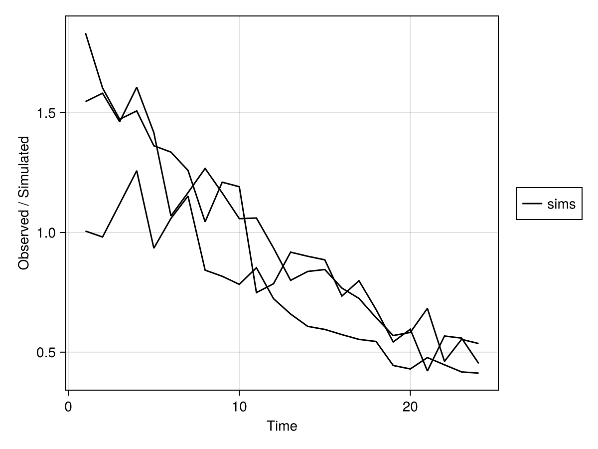

This generates a plot for each variable(s) specified in observations keyword. For example, sim_plot(m, obs; observations=[:dv1, :dv2]) would only plot the values dv1 and dv2. In addition, all the specified attributes can be used in this plot command. For more advanced use of the underlying plotting ecosystem, please see the Makie layout tutorial. Note that if the simulated return is a SimulatedPopulation, then the plots overlay the results of the various subjects.

To generate the DataFrame associated with the observed outputs, simply call DataFrame on the simulated return. For example, the following builds the tabular output from the returned object:

df = DataFrame(sims)
first(df, 5)

5×16 DataFrame

Row	id	time	dv	evid	amt	cmt	rate	duration	ss	ii	route	Central	CL	Vc	η_1	η_2
	String	Float64	Float64?	Int64	Float64?	Symbol?	Float64?	Float64?	Int8?	Float64?	NCA.Route?	Float64?	Float64?	Float64?	Float64	Float64
1	1	0.0	missing	1	100.0	Central	0.0	0.0	0	0.0	NullRoute	missing	3.31311	78.1868	0.0992754	0.264757
2	1	1.0	1.2759	0	missing	missing	missing	missing	missing	missing	missing	95.8511	3.31311	78.1868	0.0992754	0.264757
3	1	2.0	0.9999	0	missing	missing	missing	missing	missing	missing	missing	91.8743	3.31311	78.1868	0.0992754	0.264757
4	1	3.0	1.42134	0	missing	missing	missing	missing	missing	missing	missing	88.0625	3.31311	78.1868	0.0992754	0.264757
5	1	4.0	1.14577	0	missing	missing	missing	missing	missing	missing	missing	84.4089	3.31311	78.1868	0.0992754	0.264757

Different usage patterns of `simobs`

Below, we showcase the different usage patterns of simobs.

Subject level simulation

In this pattern, you can use simobs to do a single subject simulation by passing a Subject instead of a Population:

sims2 = simobs(onecomp, pop[1], ext_param; obstimes = 1:24)

SimulatedObservations
  Simulated variables: dv
  Time: 1:24

where, onecomp is the model, pop[1] represents one subject in the Population, pop. The parameters of the model are passed in as the NamedTuple defined earlier.

Subject level simulation with passing random effects

In this pattern, you can use simobs to do a single subject simulation by passing an additional positional argument of individual subject random effects represented as vector. The length of the random effect vector should be the same as the number of parameters for each subject:

ext_randeffs = (; η = [0.7, -0.44])
sims3 = simobs(onecomp, pop[1], ext_param, ext_randeffs; obstimes = 1:24)

SimulatedObservations
  Simulated variables: dv
  Time: 1:24

where, onecomp is the model, pop[1] represents one subject in the Population, pop. The parameters of the model are passed in as the NamedTuple defined earlier. ext_randeffs are the specific values of the η's that are passed in, which means that simobs uses these values as opposed to those sampled from the distributions specified in the @random block.

Subject level simulation with passing in an array of parameters

In this pattern, you can use simobs to do a single subject simulation by passing a positional argument, an array of parameters that generates a unique simulation solution for each element of the parameter array. E.g. let's simulate pop[1] with three different combinations of tvcl and tvvc. In the example below, we change the value of tvcl to represent lo, med, hi of 3, 6, 9, but we don't change the other values (Note that are more efficient programmatic ways to generate such arrays) using the syntax below:

ext_param_array = [
    (tvcl = 3, tvvc = 60, Ω = Diagonal([0.04, 0.04]), σ = 0.1),
    (tvcl = 6, tvvc = 60, Ω = Diagonal([0.04, 0.04]), σ = 0.1),
    (tvcl = 9, tvvc = 60, Ω = Diagonal([0.04, 0.04]), σ = 0.1),
]
sims4 = simobs(onecomp, pop[1], ext_param_array; obstimes = 1:24)

Simulated population (Vector{<:Subject})
  Simulated subjects: 3
  Simulated variables: dv

where, onecomp is the model, pop[1] represents one subject in the Population, pop. The parameters of the model are passed in as the vector of NamedTuples ext_param_array.

Tip

A DataFrame of parameter values can be converted to a NamedTuple easily using Tables.rowtable syntax. See the example below.

myparams = DataFrame(;
    tvcl = [1, 2, 3],
    tvvc = [20, 30, 40],
    Ω = [Diagonal([0.04, 0.04]), Diagonal([0.04, 0.04]), Diagonal([0.04, 0.04])],
    σ = 0.1,
)

3×4 DataFrame

Row	tvcl	tvvc	Ω	σ
	Int64	Int64	Diagonal…	Float64
1	1	20	[0.04 0.0; 0.0 0.04]	0.1
2	2	30	[0.04 0.0; 0.0 0.04]	0.1
3	3	40	[0.04 0.0; 0.0 0.04]	0.1

This can be converted to a NamedTuple

myparam_tuple = Tables.rowtable(myparams)

3-element Vector{@NamedTuple{tvcl::Int64, tvvc::Int64, Ω::Diagonal{Float64, Vector{Float64}}, σ::Float64}}:
 (tvcl = 1, tvvc = 20, Ω = [0.04 0.0; 0.0 0.04], σ = 0.1)
 (tvcl = 2, tvvc = 30, Ω = [0.04 0.0; 0.0 0.04], σ = 0.1)
 (tvcl = 3, tvvc = 40, Ω = [0.04 0.0; 0.0 0.04], σ = 0.1)

myparam_tuple is of the same form as the ext_param_array.

Subject level simulation with passing in an array of parameters and random effects

The two usage patterns above can be combined such that one can pass in an array of parameters and corresponding random effects with the usage pattern below:

ext_randeffs = [(; η = [0.7, -0.44]), (; η = [0.6, -0.9]), (; η = [-0.7, 0.6])]
sims5 = simobs(onecomp, pop[1], ext_param_array, ext_randeffs; obstimes = 1:24)

Simulated population (Vector{<:Subject})
  Simulated subjects: 3
  Simulated variables: dv

Population level simulations

In this pattern, you can use simobs to do a whole population simulation by passing a Population instead of a Subject:

sims6 = simobs(onecomp, pop, ext_param; obstimes = 1:24)

Simulated population (Vector{<:Subject})
  Simulated subjects: 3
  Simulated variables: dv

where, onecomp is the model, pop is the Population. The parameters of the model are passed in as the NamedTuple defined earlier.

Population level simulation passing random effects

In this pattern, you can use simobs to do a population simulation by passing an additional positional argument of individual subject random effects represented as vector. The length of the random effect vector should be the same as the number of parameters for each subject:

Tip

You can use this method to pass in the empirical_bayes of a FittedPumasModel.

ext_randeffs = [(; η = rand(2)), (; η = rand(2)), (; η = rand(2))]
sims8 = simobs(onecomp, pop, ext_param, ext_randeffs; obstimes = 1:24)

Simulated population (Vector{<:Subject})
  Simulated subjects: 3
  Simulated variables: dv

where, onecomp is the model, pop represents the Population, pop. The parameters of the model are explicitly passed in as the NamedTuple defined earlier. ext_randeffs are the specific values of the η's that are passed in, which means that simobs uses these values as opposed to those sampled from the distributions specified in the @random block.

Population level simulation with passing in an array of parameters

The two usage patterns above can be combined such that one can pass in an array of parameters and corresponding random effects.

Here, a population can be simulated with an array of parameters that generates a unique simulation solution for each element of the parameter array. E.g. let's simulate pop with three different combinations of tvcl and tvvc. In the example below, we change the value of tvcl to represent lo, med, hi of 3, 6, 9, but we don't change the other values (Note that are more efficient programmatic ways to generate such arrays):

ext_param_array = [
    (; tvcl = 3, tvvc = 60, Ω = Diagonal([0.04, 0.04]), σ = 0.1),
    (; tvcl = 6, tvvc = 60, Ω = Diagonal([0.04, 0.04]), σ = 0.1),
    (; tvcl = 9, tvvc = 60, Ω = Diagonal([0.04, 0.04]), σ = 0.1),
]
sims9 = simobs(onecomp, pop, ext_param_array; obstimes = 1:24)

3-element Vector{Vector{Pumas.SimulatedObservations{PumasModel{(tvcl = 1, tvvc = 1, Ω = 2, σ = 1), 2, (:Central,), (:CL, :Vc), ParamSet{@NamedTuple{tvcl::RealDomain{Int64, TransformVariables.Infinity{true}, Int64}, tvvc::RealDomain{Int64, TransformVariables.Infinity{true}, Int64}, Ω::PDiagDomain{PDMats.PDiagMat{Float64, Vector{Float64}}}, σ::RealDomain{Float64, TransformVariables.Infinity{true}, Float64}}}, Main.var"#1#6", Main.var"#2#7", Nothing, Main.var"#3#8", Central1, Pumas.DerivedObj{(:dv,), Main.var"#4#9"}, Main.var"#5#10", Nothing, Pumas.PumasModelOptions}, Subject{@NamedTuple{dv::Vector{Missing}}, Pumas.ConstantCovar{@NamedTuple{}}, DosageRegimen{Float64, Symbol, Float64, Float64, Float64, Float64}, Nothing}, UnitRange{Int64}, @NamedTuple{tvcl::Int64, tvvc::Int64, Ω::Diagonal{Float64, Vector{Float64}}, σ::Float64}, @NamedTuple{η::Vector{Float64}}, @NamedTuple{}, @NamedTuple{callback::Nothing, continuity::Symbol, saveat::UnitRange{Int64}, alg::CompositeAlgorithm{1, Tuple{OrdinaryDiffEq.Tsit5{typeof(OrdinaryDiffEq.trivial_limiter!), typeof(OrdinaryDiffEq.trivial_limiter!), Static.False}, Rosenbrock23{1, true, LinearSolve.GenericLUFactorization{LinearAlgebra.RowMaximum}, typeof(OrdinaryDiffEq.DEFAULT_PRECS), Val{:forward}, true, nothing, typeof(OrdinaryDiffEq.trivial_limiter!), typeof(OrdinaryDiffEq.trivial_limiter!)}}, OrdinaryDiffEq.AutoSwitch{OrdinaryDiffEq.Tsit5{typeof(OrdinaryDiffEq.trivial_limiter!), typeof(OrdinaryDiffEq.trivial_limiter!), Static.False}, Rosenbrock23{1, true, LinearSolve.GenericLUFactorization{LinearAlgebra.RowMaximum}, typeof(OrdinaryDiffEq.DEFAULT_PRECS), Val{:forward}, true, nothing, typeof(OrdinaryDiffEq.trivial_limiter!), typeof(OrdinaryDiffEq.trivial_limiter!)}, Rational{Int64}, Int64}}}, Pumas.PKPDAnalyticalSolution{StaticArraysCore.SVector{1, Float64}, 2, Vector{StaticArraysCore.SVector{1, Float64}}, Vector{Float64}, Vector{StaticArraysCore.SVector{1, Float64}}, Vector{StaticArraysCore.SVector{1, Float64}}, Returns{@NamedTuple{CL::Float64, Vc::Float64}}, Pumas.AnalyticalPKPDProblem{StaticArraysCore.SVector{1, Float64}, Float64, false, Central1, Vector{Pumas.Event{Float64, Float64, Float64}}, Vector{Float64}, Returns{@NamedTuple{CL::Float64, Vc::Float64}}}}, @NamedTuple{}, @NamedTuple{CL::Vector{Float64}, Vc::Vector{Float64}}, @NamedTuple{dv::Vector{Float64}}, @NamedTuple{}}}}:
 Simulated population (Vector{<:Subject}), n = 3, variables: dv
 Simulated population (Vector{<:Subject}), n = 3, variables: dv
 Simulated population (Vector{<:Subject}), n = 3, variables: dv

where, onecomp is the model, pop represents the Population, pop. The parameters of the model are passed in as a vector of the NamedTuples ext_param_array as defined earlier represents the array of parameter values we want to simulate the model at.

Population level simulation with passing in an array of parameters and random effects

The two usage patterns above can be combined such that one can pass in an array of parameters and corresponding random effects with the usage pattern below:

ext_randeffs_array = [(; η = rand(2)) for i = 1:length(ext_param_array)*length(pop)]
sims10 = simobs(onecomp, pop, ext_param_array, ext_randeffs_array; obstimes = 1:24)

3-element Vector{Vector{Pumas.SimulatedObservations{PumasModel{(tvcl = 1, tvvc = 1, Ω = 2, σ = 1), 2, (:Central,), (:CL, :Vc), ParamSet{@NamedTuple{tvcl::RealDomain{Int64, TransformVariables.Infinity{true}, Int64}, tvvc::RealDomain{Int64, TransformVariables.Infinity{true}, Int64}, Ω::PDiagDomain{PDMats.PDiagMat{Float64, Vector{Float64}}}, σ::RealDomain{Float64, TransformVariables.Infinity{true}, Float64}}}, Main.var"#1#6", Main.var"#2#7", Nothing, Main.var"#3#8", Central1, Pumas.DerivedObj{(:dv,), Main.var"#4#9"}, Main.var"#5#10", Nothing, Pumas.PumasModelOptions}, Subject{@NamedTuple{dv::Vector{Missing}}, Pumas.ConstantCovar{@NamedTuple{}}, DosageRegimen{Float64, Symbol, Float64, Float64, Float64, Float64}, Nothing}, UnitRange{Int64}, @NamedTuple{tvcl::Int64, tvvc::Int64, Ω::Diagonal{Float64, Vector{Float64}}, σ::Float64}, @NamedTuple{η::Vector{Float64}}, @NamedTuple{}, @NamedTuple{callback::Nothing, continuity::Symbol, saveat::UnitRange{Int64}, alg::CompositeAlgorithm{1, Tuple{OrdinaryDiffEq.Tsit5{typeof(OrdinaryDiffEq.trivial_limiter!), typeof(OrdinaryDiffEq.trivial_limiter!), Static.False}, Rosenbrock23{1, true, LinearSolve.GenericLUFactorization{LinearAlgebra.RowMaximum}, typeof(OrdinaryDiffEq.DEFAULT_PRECS), Val{:forward}, true, nothing, typeof(OrdinaryDiffEq.trivial_limiter!), typeof(OrdinaryDiffEq.trivial_limiter!)}}, OrdinaryDiffEq.AutoSwitch{OrdinaryDiffEq.Tsit5{typeof(OrdinaryDiffEq.trivial_limiter!), typeof(OrdinaryDiffEq.trivial_limiter!), Static.False}, Rosenbrock23{1, true, LinearSolve.GenericLUFactorization{LinearAlgebra.RowMaximum}, typeof(OrdinaryDiffEq.DEFAULT_PRECS), Val{:forward}, true, nothing, typeof(OrdinaryDiffEq.trivial_limiter!), typeof(OrdinaryDiffEq.trivial_limiter!)}, Rational{Int64}, Int64}}}, Pumas.PKPDAnalyticalSolution{StaticArraysCore.SVector{1, Float64}, 2, Vector{StaticArraysCore.SVector{1, Float64}}, Vector{Float64}, Vector{StaticArraysCore.SVector{1, Float64}}, Vector{StaticArraysCore.SVector{1, Float64}}, Returns{@NamedTuple{CL::Float64, Vc::Float64}}, Pumas.AnalyticalPKPDProblem{StaticArraysCore.SVector{1, Float64}, Float64, false, Central1, Vector{Pumas.Event{Float64, Float64, Float64}}, Vector{Float64}, Returns{@NamedTuple{CL::Float64, Vc::Float64}}}}, @NamedTuple{}, @NamedTuple{CL::Vector{Float64}, Vc::Vector{Float64}}, @NamedTuple{dv::Vector{Float64}}, @NamedTuple{}}}}:
 Simulated population (Vector{<:Subject}), n = 3, variables: dv
 Simulated population (Vector{<:Subject}), n = 3, variables: dv
 Simulated population (Vector{<:Subject}), n = 3, variables: dv

Simulation using a `FittedPumasModelInference`

The usage pattern is represented below:

Pumas.simobs — Method

simobs(pmi::FittedPumasModelInference, population::Population = pmi.fpm.data, randeffs::Union{Nothing, AbstractVector{<:NamedTuple}} = nothing; samples::Int, rng = default_rng(), kwargs...,)

Any model that has been fitted results in a FittedPumasModelInference. simobs can simulate from the inferred object where it utilizes the variance-covariance-matrix of the infer and the design of the data that was fitted.

Post-processing simulations

The output of a simobs call stores the simulated observations but also all the intermediate values computed such as the parameters used, individual coefficients, dose control parameters, covariates, differential equation solution, etc. There are a number of post-processing operations you can do on the simulation output to compute various queries and summary statistics based on the simulations.

The postprocess function is a powerful tool that allows you to make various queries using the simulation results.

Pumas.postprocess — Function

postprocess(obs::SimulatedObservations)
postprocess(func::Function, obs::SimulatedObservations)
postprocess(obs::SimulatedPopulation; stat = identity)
postprocess(func::Function, obs::SimulatedPopulation; stat = identity)

Post-processes the output of simobs. The output of a simobs call stores the simulated observations but also all the intermediate values computed such as the parameters used, individual coefficients, dose control parameters, covariates, differential equation solution, etc. There are a number of post-processing operations you can do on the simulation output to compute various queries and summary statistics based on the simulations.

The postprocess function is a powerful tool that allows you to make various queries using the simulation results. There are multiple ways to use the postprocess function. The first way to use the postprocess function is to extract all the information stored in the simulation result in the form of a vector of named tuples. Each named tuple has all the intermediate values evaluated when simulating 1 run. Let sims be the output of any simobs operation.

generated = Pumas.postprocess(sims)

generated is a vector of simulation runs. Hence, generated[i] is the result from the ith simulation run. Time-dependent variables are stored as a vector with 1 element for each time point where there is an observation. Alternatively, if obstimes was set instead when calling simobs, the time-dependent variables will be evaluated at the time points in obstimes instead.

The second way to use postprocess is by passing in a post-processing function. The post-processing function can be used to:

Transform the simulated quantities, or
Compare the simulated quantities to the observations.

We use the do syntax here which is short for passing in a function as the first argument to postprocess. The do syntax to pass in a post-processing function is:

Pumas.postprocess(sims) do gen, obs
  ...
end

where gen is the named tuple of all generated quantities from 1 simulation run and obs is the named tuple of observations. For instance to query the ratio of simulated observations dv that are higher than the observed quantity dv at the respective time points, you can use:

Pumas.postprocess(sims) do gen, obs
  sum(gen.dv .> obs.dv) / length(gen.dv)
end

gen.dv is the simulated vector of dv whose length is the same as the number of observation time points. obs.dv is the observation vector dv. gen.dv .> obs.dv returns a vector of true/false, with one element for each time point. The sum of this vector gives the number of time points where the simulation was higher than the observation. Dividing by the number of time points gives the ratio. When using postprocess in this way, the output is always a vector of the query results. In the query function body, you can choose to use only gen or only obs but the header must always have both gen and obs:

Pumas.postprocess(sims) do gen, obs
  ...
end

The third way to use the postprocess function is to compute summary statistics of the simulated quantities or of functions of the simulated quantities. Summary statistics can be computed by passing a statistic function as the stat keyword argument. For example in order to estimate the probability that a simulated value is higher than an observation, you can use:

Pumas.postprocess(sims, stat = mean) do gen, obs
  gen.dv .> obs.dv
end

This function will do 2 things:

Concatenate the query results (e.g. gen.dv .> obs.dv) from all the simulation runs into a single vector.
Compute the mean value of the combined vector.

Alternatively, you can use the mean function to do the same thing without using the keyword argument. The following will call the postprocess function under the hood.

mean(sims) do gen, obs
  gen.dv .> obs.dv
end

The result of this operation will be a scalar equal to the mean value of the concatenated vector of queries.

In order to get the probability that the simulated quantity is higher than the observation for each time point, you can call the mean function externally as such:

generated = Pumas.postprocess(sims) do gen, obs
  gen.dv .> obs.dv
end
mean(generated)

This returns a vector of probabilities of the same length as the number of time points without concatenating all the queries together.

To compute a summary statistic of all the generated quantity, you can also call:

Pumas.postprocess(sims, stat = mean)

without specifying a post-processing function or for short:

mean(sims)

Besides mean, you can also use any of the following summary statistic functions in the same way:

std for element-wise standard deviation
var for element-wise variance
cor for correlation between multiple quantities
cov for covariance between multiple quantities

These functions can be passed in as the stat keyword argument to postprocess or they can be used in the short form, e.g.:

generated = Pumas.postprocess(sims, stat = std) do gen, obs
  ...
end
std(sims) do gen, obs
  ...
end
std(sims)

generated = Pumas.postprocess(sims, stat = var) do gen, obs
  ...
end
var(sims) do gen, obs
  ...
end
var(sims)

The cor and cov statistics are unique in that they require a post-processing function that outputs a vector. For example, to estimate the correlation between the CL and Vc parameters in a 1-compartment model, you can use any of the following:

Pumas.postprocess(s, stat = cor) do gen, obs
  [gen.CL[1], gen.Vc[1]]
end
cor(s) do gen, obs
  [gen.CL[1], gen.Vc[1]]
end

Note that gen.CL is a vector of simulated CL values for all the time points. But since the value is constant across time, we can use the first element gen.CL[1] only. cov can be used instead of cor to compute the covariance matrix. The output of this operation is either a correlation or a covariance matrix.