Covariate Modeling

Pumas can handle subject covariates, both time-varying and constant. They are handled inside the @covariates model block and parsed in a Population with the covariates keyword argument from the read_pumas function.

Let's show an example with the nlme_sample dataset from thePharmaDatasets package:

using Pumas
using PharmaDatasets
using DataFrames

pkdata = dataset("nlme_sample")
describe(pkdata)

pkdata here is an intravenous infusion given over 2 hours with demographic information (age, weight, sex, and creating clearance). The first thing we need to do is to parse pkdata into a Population with read_pumas while adding the desired columns to be parsed as covariates in the covariates keyword argument:

pop = read_pumas(
    pkdata;
    id = :ID,
    time = :TIME,
    amt = :AMT,
    covariates = [:WT, :AGE, :SEX, :CRCL, :GROUP],
    observations = [:DV],
    cmt = :CMT,
    evid = :EVID,
    rate = :RATE,
)

Population
  Subjects: 30
  Covariates: WT, AGE, SEX, CRCL, GROUP
  Observations: DV

For the model part, we need to declare the covariates in the @covariates model block. Then, we can use it in the @pre and @dosecontrol blocks. Here's a two-compartment combined-error model that uses WT as a covariate in allometric scaling of both CL and Vc PK parameters:

model = @model begin
    @param begin
        tvcl ∈ RealDomain(; lower = 0)
        tvvc ∈ RealDomain(; lower = 0)
        tvq ∈ RealDomain(; lower = 0)
        tvvp ∈ RealDomain(; lower = 0)
        Ω ∈ PDiagDomain(2)
        σ²_add ∈ RealDomain(; lower = 0)
        σ²_prop ∈ RealDomain(; lower = 0)
    end

    @random begin
        η ~ MvNormal(Ω)
    end

    @covariates WT

    @pre begin
        wtCL = (WT / 70)^0.75
        wtV = (WT / 70)
        CL = tvcl * wtCL * exp(η[1])
        Vc = tvvc * wtV * exp(η[2])
        Q = tvq
        Vp = tvvp
    end

    @dynamics Central1Periph1

    @derived begin
        cp := @. Central / Vc
        DV ~ @. Normal(cp, sqrt(abs(cp)^2 * σ²_prop + σ²_add))
    end
end

PumasModel
  Parameters: tvcl, tvvc, tvq, tvvp, Ω, σ²_add, σ²_prop
  Random effects: η
  Covariates: WT
  Dynamical system variables: Central, Peripheral
  Dynamical system type: Closed form
  Derived: DV
  Observed: DV

We first declare WT in the @covariates block then we are free to use WT in the @pre block.

Now an example with multiple covariates:

model_multiple = @model begin
    @param begin
        tvcl ∈ RealDomain(; lower = 0)
        tvvc ∈ RealDomain(; lower = 0)
        tvq ∈ RealDomain(; lower = 0)
        tvvp ∈ RealDomain(; lower = 0)
        Ω ∈ PDiagDomain(2)
        σ²_add ∈ RealDomain(; lower = 0)
        σ²_prop ∈ RealDomain(; lower = 0)
    end

    @random begin
        η ~ MvNormal(Ω)
    end

    @covariates begin
        WT
        CRCL
    end

    @pre begin
        wtCL = (WT / 70)^0.75
        wtV = (WT / 70)
        crcl_eff = (CRCL / 95)^0.75
        CL = tvcl * wtCL * crcl_eff * exp(η[1])
        Vc = tvvc * wtV * exp(η[2])
        Q = tvq
        Vp = tvvp
    end

    @dynamics Central1Periph1

    @derived begin
        cp := @. Central / Vc
        DV ~ @. Normal(cp, sqrt(abs(cp)^2 * σ²_prop + σ²_add))
    end
end

PumasModel
  Parameters: tvcl, tvvc, tvq, tvvp, Ω, σ²_add, σ²_prop
  Random effects: η
  Covariates: WT, CRCL
  Dynamical system variables: Central, Peripheral
  Dynamical system type: Closed form
  Derived: DV
  Observed: DV

The @covariates model block, like other Pumas' model blocks, supports one statement per line inside begin ... end.

Creating Binary Covariates

You can use binary covariates inside a Pumas model using either ifelse function or the ternary operator ?. The nlme_sample dataset has the following values for the :SEX column:

unique(pkdata.SEX)

2-element Vector{InlineStrings.String1}:
 "M"
 "F"

Here's an example where we are using different residual unexplained variance (the σ²s parameters) for each unique value of :SEX:

model_multiple_errors = @model begin
    @param begin
        tvcl ∈ RealDomain(; lower = 0)
        tvvc ∈ RealDomain(; lower = 0)
        tvq ∈ RealDomain(; lower = 0)
        tvvp ∈ RealDomain(; lower = 0)
        Ω ∈ PDiagDomain(2)
        σ²_add_F ∈ RealDomain(; lower = 0)
        σ²_prop_F ∈ RealDomain(; lower = 0)
        σ²_add_M ∈ RealDomain(; lower = 0)
        σ²_prop_M ∈ RealDomain(; lower = 0)
    end

    @random begin
        η ~ MvNormal(Ω)
    end

    @covariates SEX

    @pre begin
        CL = tvcl * exp(η[1])
        Vc = tvvc * exp(η[2])
        Q = tvq
        Vp = tvvp

        # a different σ for SEX
        σ²_add = ifelse(SEX == "M", σ²_add_M, σ²_add_F)
        σ²_prop = ifelse(SEX == "M", σ²_prop_M, σ²_prop_F)
    end

    @dynamics Central1Periph1

    @derived begin
        cp := @. Central / Vc
        DV ~ @. Normal(cp, sqrt(abs(cp)^2 * σ²_prop + σ²_add))
    end
end

PumasModel
  Parameters: tvcl, tvvc, tvq, tvvp, Ω, σ²_add_F, σ²_prop_F, σ²_add_M, σ²_prop_M
  Random effects: η
  Covariates: SEX
  Dynamical system variables: Central, Peripheral
  Dynamical system type: Closed form
  Derived: DV
  Observed: DV

You can nest as many ifelse statements as needed if your covariate has more than 2 categories. For example with :GROUP column:

unique(pkdata.GROUP)

3-element Vector{InlineStrings.String7}:
 "1000 mg"
 "750 mg"
 "500 mg"

You perform the following nested ifelse:

σ = ifelse(GROUP == "500mg", σ_500, ifelse(GROUP == "750mg", σ_750, σ_1000))

Covariates with Coefficients

Some covariates need coefficients. In Pumas models, this can be accomplished by adding the coefficient in the @param block, the covariate in the @covariates block, and the pre-computation of the covariate effect in the @pre block. Here's an example of a linear relationship with no intercept:

@param begin
    tvcovar ∈ RealDomain() # the covariate effect coefficient
end

@covariates COVAR

@pre begin
    COVAR_effect = tvcovar * COVAR
end

Passing Covariates to Other Pumas Model Blocks

Covariates specified in the @covariates block can only be used in the @pre and @dosecontrol blocks. However, users might want to use covariates in other model blocks such as the @derived block. For that, you can create a variable inside the @pre block that is equal to the desired covariate. This variable, like all variables defined in the @pre block, is available for all other model blocks to use. Hence, in the desired model block, you can use the covariate by first passing it through the @pre block:

@covariates COVAR

@pre begin
    _COVAR = COVAR
end

@derived begin
    # you can freely use _COVAR here
end

Fitting Covariate Models

Covariate model fitting is the same as any other Pumas model fitting. You'll need to pass the required positional arguments to the fit function:

1. model
2. population
3. initial parameter values
4. estimation method

iparams = (;
    tvvc = 5,
    tvcl = 0.02,
    tvq = 0.01,
    tvvp = 10,
    Ω = Diagonal([0.01, 0.01]),
    σ²_add = 0.01,
    σ²_prop = 0.01,
)

(tvvc = 5,
 tvcl = 0.02,
 tvq = 0.01,
 tvvp = 10,
 Ω = [0.01 0.0; 0.0 0.01],
 σ²_add = 0.01,
 σ²_prop = 0.01,)

model_fit = fit(
    model_multiple,
    pop,
    iparams,
    FOCE();
    # hide the trace output during fitting
    optimize_fn = Pumas.DefaultOptimizeFN(; show_trace = false),
)

FittedPumasModel

Successful minimization:                      true

Likelihood approximation:                     FOCE
Likelihood Optimizer:                         BFGS
Dynamical system type:                 Closed form

Log-likelihood value:                    -1891.253
Number of subjects:                             30
Number of parameters:         Fixed      Optimized
                                  0              8
Observation records:         Active        Missing
    DV:                         540              0
    Total:                      540              0

-----------------------
            Estimate
-----------------------
tvcl         0.1788
tvvc         3.9762
tvq          0.042664
tvvp         3.8242
Ω₁,₁         0.17121
Ω₂,₂         0.081303
σ²_add       0.0010351
σ²_prop      0.0037221
-----------------------

Annotating Covariates

Users can also annotate covariates inside the @covariates block by adding a string before the covariate. For example:

model_annotated = @model begin
    @param begin
        tvcl ∈ RealDomain(; lower = 0)
        tvvc ∈ RealDomain(; lower = 0)
        tvq ∈ RealDomain(; lower = 0)
        tvvp ∈ RealDomain(; lower = 0)
        Ω ∈ PDiagDomain(2)
        σ²_add ∈ RealDomain(; lower = 0)
        σ²_prop ∈ RealDomain(; lower = 0)
    end

    @random begin
        η ~ MvNormal(Ω)
    end

    @covariates begin
        """
        Weight
        """
        WT
        """
        Creatine Clearance
        """
        CRCL
    end

    @pre begin
        wtCL = (WT / 70)^0.75
        wtV = (WT / 70)
        crcl_eff = (CRCL / 95)^0.75
        CL = tvcl * wtCL * crcl_eff * exp(η[1])
        Vc = tvvc * wtV * exp(η[2])
        Q = tvq
        Vp = tvvp
    end

    @dynamics Central1Periph1

    @derived begin
        cp := @. Central / Vc
        DV ~ @. Normal(cp, sqrt(abs(cp)^2 * σ²_prop + σ²_add))
    end
end

PumasModel
  Parameters: tvcl, tvvc, tvq, tvvp, Ω, σ²_add, σ²_prop
  Random effects: η
  Covariates: WT, CRCL
  Dynamical system variables: Central, Peripheral
  Dynamical system type: Closed form
  Derived: DV
  Observed: DV

Most of the Pumas functions and plots will use the annotated information in their output:

model_annotated_fit = fit(
    model_annotated,
    pop,
    iparams,
    FOCE();
    # hide the trace output during fitting
    optimize_fn = Pumas.DefaultOptimizeFN(; show_trace = false),
)

FittedPumasModel

Successful minimization:                      true

Likelihood approximation:                     FOCE
Likelihood Optimizer:                         BFGS
Dynamical system type:                 Closed form

Log-likelihood value:                    -1891.253
Number of subjects:                             30
Number of parameters:         Fixed      Optimized
                                  0              8
Observation records:         Active        Missing
    DV:                         540              0
    Total:                      540              0

-----------------------
            Estimate
-----------------------
tvcl         0.1788
tvvc         3.9762
tvq          0.042664
tvvp         3.8242
Ω₁,₁         0.17121
Ω₂,₂         0.081303
σ²_add       0.0010351
σ²_prop      0.0037221
-----------------------

model_inspect = inspect(model_annotated_fit)

FittedPumasModelInspection

Fitting was successful: true
Likehood approximation used for weighted residuals : FOCE{Optim.NewtonTrustRegion{Float64}, Optim.Options{Float64, Nothing}}(Optim.NewtonTrustRegion{Float64}(1.0, 100.0, 1.4901161193847656e-8, 0.1, 0.25, 0.75, false), Optim.Options(x_abstol = 0.0, x_reltol = 0.0, f_abstol = 0.0, f_reltol = 0.0, g_abstol = 1.0e-5, g_reltol = 1.0e-8, outer_x_abstol = 0.0, outer_x_reltol = 0.0, outer_f_abstol = 0.0, outer_f_reltol = 0.0, outer_g_abstol = 1.0e-8, outer_g_reltol = 1.0e-8, f_calls_limit = 0, g_calls_limit = 0, h_calls_limit = 0, allow_f_increases = false, allow_outer_f_increases = true, successive_f_tol = 1, iterations = 1000, outer_iterations = 1000, store_trace = false, trace_simplex = false, show_trace = false, extended_trace = false, show_every = 1, time_limit = NaN, )
)

using PumasUtilities

empirical_bayes_vs_covariates(model_inspect)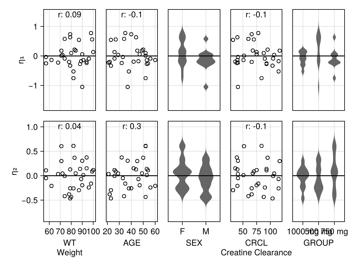

As you can see WT and CRCL which were annotated in our Pumas model has enhanced labels in empirical_bayes_vs_covariates.

Additionally, notice that even if our model specifies only two covariates, empirical_bayes_vs_covariates uses the underlying information in the Population that the model was fitted to plot all the remaining covariates along with the ones the model specifies.

Time-varying Covariates

Pumas can handle time-varying covariates. This happens automatically if, when parsing a dataset, read_pumas detects that covariate values change over time.

Here's an example with an ordinal regression using the painord dataset from PharmaDatasets. :painord is our observations measuring the perceived pain in a scale from 0 to 3, which we need to have the range shifted by 1 (1 to 4). Additionally, we'll use the concentration in plasma, :conc as a covariate. Of course, :conc varies with time, thus, it is a time-varying covariate:

using Pumas
using PharmaDatasets
using DataFrames

painord = dataset("pumas/pain_remed")
describe(painord)

using DataFramesMeta

@rtransform! painord :painord = :painord + 1

pop =
    read_pumas(painord; observations = [:painord], covariates = [:conc], event_data = false)

160-element Vector{Subject{NamedTuple{(:painord,), Tuple{Vector{Union{Missing, Float64}}}}, T2, Nothing, Vector{Float64}} where T2}:
 Subject(id = 1, ...)
 Subject(id = 2, ...)
 Subject(id = 3, ...)
 Subject(id = 4, ...)
 Subject(id = 5, ...)
 Subject(id = 6, ...)
 Subject(id = 7, ...)
 Subject(id = 8, ...)
 Subject(id = 9, ...)
 Subject(id = 10, ...)
 Subject(id = 11, ...)
 Subject(id = 12, ...)
 Subject(id = 13, ...)
 ⋮
 Subject(id = 149, ...)
 Subject(id = 150, ...)
 Subject(id = 151, ...)
 Subject(id = 152, ...)
 Subject(id = 153, ...)
 Subject(id = 154, ...)
 Subject(id = 155, ...)
 Subject(id = 156, ...)
 Subject(id = 157, ...)
 Subject(id = 158, ...)
 Subject(id = 159, ...)
 Subject(id = 160, ...)

The following model uses the Categorical distribution inside the @derived for our observation :painord. There are also some computations in the @pre block to calculate the log-cumulative-odds and probabilities for each categorical value:

ordinal_model = @model begin
    @param begin
        b₁ ∈ RealDomain(; init = 0)
        b₂ ∈ RealDomain(; init = 1)
        b₃ ∈ RealDomain(; init = 1)
        slope ∈ RealDomain(; init = 0)
    end

    @covariates conc # time varying

    @pre begin
        effect = slope * conc

        # Logit of cumulative probabilities
        lge₁ = b₁ + effect
        lge₂ = lge₁ - b₂
        lge₃ = lge₂ - b₃

        # Probabilities of >=1 and >=2 and >=3
        pge₁ = logistic(lge₁)
        pge₂ = logistic(lge₂)
        pge₃ = logistic(lge₃)

        # Probabilities of Y=1,2,3,4
        p₁ = 1.0 - pge₁
        p₂ = pge₁ - pge₂
        p₃ = pge₂ - pge₃
        p₄ = pge₃
    end

    @derived begin
        painord ~ @. Categorical(p₁, p₂, p₃, p₄)
    end
end

PumasModel
  Parameters: b₁, b₂, b₃, slope
  Random effects: 
  Covariates: conc
  Dynamical system variables: 
  Dynamical system type: No dynamical model
  Derived: painord
  Observed: painord

As expected this model fits without problems using NaivePooled as an estimation method:

ordinal_fit = fit(
    ordinal_model,
    pop,
    init_params(ordinal_model),
    NaivePooled();
    # hide the trace output during fitting
    optimize_fn = Pumas.DefaultOptimizeFN(; show_trace = false),
)

FittedPumasModel

Successful minimization:                      true

Likelihood approximation:              NaivePooled
Likelihood Optimizer:                         BFGS
Dynamical system type:          No dynamical model

Log-likelihood value:                   -2316.3554
Number of subjects:                            160
Number of parameters:         Fixed      Optimized
                                  0              4
Observation records:         Active        Missing
    painord:                   1920              0
    Total:                     1920              0

-------------------
          Estimate
-------------------
b₁         2.5112
b₂         2.1951
b₃         1.9643
slope     -0.38871
-------------------

Missing Values in Covariates

The way that Pumas handles missing values inside covariates depends on whether the covariate is constant or time-varying. For both cases Pumas will interpolate the available values to fill in the missing values. If, for any subject, all the covariate's values are missing, Pumas will throw an error while parsing the data with read_pumas.

For both missing constant and time-varying covariates, Pumas, by default, does piece-wise constant interpolation with "next observation carried backward" (NOCB, NONMEM default). Of course for constant covariates the interpolated values over the missing values will be constant values. This can be adjusted with the covariates_direction keyword argument of read_pumas. The default value :right is NOCB and :left is "last observation carried forward" (LOCF, Monolix default).

Hence, for LOCF, you can use the following:

pop = read_pumas(pkdata; covariates_direction = :left)

along with any other required keyword arguments for column mapping.