Bioequivalence Power Introduction
The Pumas BioequivalencePower package provides functionality for power calculation and sample size determination for bioequivalence trials. The package supports multiple study types and multiple designs. To start:
using BioequivalencePowerAs this is a new addition to Pumas, with future Pumas releases, the current API and logical structure of the package, including methods of specifying designs, and other aspects, is not guaranteed to remain as in the current version.
Overview of key functions and types
The most important functionality of BioequivalencePower is sample size determination via the function samplesize, for which there are multiple methods. Sample size determination hinges on power computation via the power function, for which there are also multiple methods.
In addition, the package exposes a few additional functions such as adjusted_α for determining the best specified $\alpha$ to achieve a given type I error (may be useful in scenarios where $\alpha$ and the Type I error do not agree), adjusted_α_with_samplesize for making such an adjustment together with sample size determination, and importantly, power_analysis for analyzing the effect of parameter miss-specification on the sample size determination and power calculations. Other useful functions are confint and pvalue, applied to specific tests, as well as multiple miscellaneous utility functions.
The BioequivalencePower package provides all the functionality available in the R language PowerTOST package (version 1.5.4). The interface and internals of the computation differ from PowerTOST, yet the functionality is essentially identical and in a few cases has more options than PowerTOST. Computations carried out by this package have been tested to yield the same output (up to a numerical and simulation margin of error) as PowerTOST. About 250,000 example power and samplesize computations were carried out to compare BioequivalencePower and PowerTOST.
Two key concepts of the package are a power study and a design. The key functions, samplesize, power, adjusted_α, adjusted_α_with_samplesize, power_analysis, confint, and pvalue are always applied to a combination of a power study and a design.
Programmatically, all the power study types are subtypes of BioequivalencePowerStudy. Note that TOST stands for "Two One Sided T-Test", and here we also use OST for "One Sided T-Test". The supported power study types are:
- Standard (average) bioequivalence:
RatioTOSTandDifferenceTOST - Reference scaling and/or expanding limits:
ReferenceScaledRatioTOST,ExpandingLimitsRatioTOST - Tests for NTID (Narrow Therapeutic Index Drug):
NarrowTherapeuticIndexDrugRatioTOST(this also includes the highly variable case) - Tests in the context of fiducial inference:
FiducialRatioTOST - Tests with two end points:
TwoDifferenceTOSTsandTwoRatioTOSTs - Tests for dose proportionality:
DoseProportionalityStudy - Non-inferiority tests:
NonInferiorityRatioOSTandNonInferiorityDifferenceOST - Bayesian Wrapping on Parameters in tests:
CVSEPrior,θ0Prior,BothCVSEandθ0Priorusing parametersDegreesOfFreedomPriorParameters,StandardErrorPriorParameters, orDegreesOfFreedomAndStandardErrorPriorParametersrespectively
Programmatically, all the design types included are subtypes of ExperimentalDesign. These types are:
Designs with 2 treatments:
Parallel design:
ED2ParallelCross over design with 2 sequences, and 2 periods:
ED2x2CrossoverCommonly used replicate cross over designs with 2 sequences, and,
- 3 periods:
ED2x2x3ReplicateCrossover - 4 periods:
ED2x2x4ReplicateCrossover
- 3 periods:
A commonly used partial replicate design with 3 sequences, and 3 periods:
ED2x3x3PartialReplicateAdditional designs:
- 4 sequences and 4 periods:
ED2x4x4ReplicateCrossover - 4 sequences and 2 periods Balaam's design:
ED2x4x2Balaam - 2 sequences and 2 periods, with 2 repeated targets determined in each period:
ED2x2x2RepeatedCrossover - A paired t-test type design:
EDPaired
- 4 sequences and 4 periods:
Designs with more than 2 treatments:
- 3 treatments, 3 sequences, and 3 periods:
ED3x3Crossover - 3 treatments, 6 sequences, and 3 periods:
ED3x6x3Crossover - 4 treatments, 4 sequences, and 4 periods:
ED4x4Crossover
Other designs types:
- Arbitrary general crossover designs:
EDGeneralCrossover - Arbitrary general parallel designs:
EDGeneralParallel - Arbitrary general designs specified by a design matrix:
EDGeneral
In addition to the types above specifying the power study and the design, another key type to the package is HypothesisTestMetaParams. This type specifies the sample size, $\alpha$, power, and similar descriptions of a study.
Basic usage
There are two APIs available for the package, which are called the easy API (also viewed as the "convenient API" or "standard API") and the complete API (also viewed as the "expert API" or "versatile API"). The standard API is useful for simple application of functions (samplesize, power, etc.) and is probably the API to be used for most applications. The complete API is the internal API used under the hood by the easy API, since the easy API is merely a wrapper on top of it. Certain advanced applications, that incorporate the package inside bigger simulation studies, may merit benefit from the use of the complete API.
Example usage of the easy API
Let us start with a simple example:
samplesize(RatioTOST, ED2Parallel, CV = 0.3, peθ₀ = 0.93)Determined sample size: n = 96 achieved power = 80.171%
HypothesisTestMetaParams Settings: α = 0.05 target_power = 0.8
Study: RatioTOST{ED2Parallel} CV = 0.3 θ₀ = 0.93 [θ₁, θ₂] = [0.8, 1.25]This is a "sample size computation" for a RatioTOST bioequivalence power study type (this is also known as basic average bioequivalence) with a parallel design. The sample size is based on an assumed CV of 30% and an assumed ratio of treatment average to reference average of 93% (more on the basics statistical principles of such tests is below). There are also default parameters at play, not explicitly specified in this example. These include α = 0.05, target_power = 0.80, and others. In the output we see that 96 subjects (48 per treatment) are needed to overcome the target power of 80%. This yields an achieved power of about 80.2%. The return type here is an object of the type HypothesisTestMetaParams.
As a sanity check you can compute the power for this case based on n = 96 subjects:
power(RatioTOST, ED2Parallel, n = 96, CV = 0.3, peθ₀ = 0.93)Computed achieved power: 80.171%
HypothesisTestMetaParams Settings: n = 96 α = 0.05
Study: RatioTOST{ED2Parallel} CV = 0.3 θ₀ = 0.93 [θ₁, θ₂] = [0.8, 1.25]You can see that achieved_power is exactly as specified when we used samplesize. Further, as a follow up analysis, assume now an unbalanced design with say 52 subjects for the first treatment and 44 subjects for the second treatment (still 96 subjects in the study):
power(RatioTOST, ED2Parallel, n = [52, 44], CV = 0.3, peθ₀ = 0.93)Computed achieved power: 79.925%
HypothesisTestMetaParams Settings: n = [52, 44] α = 0.05
Study: RatioTOST{ED2Parallel} CV = 0.3 θ₀ = 0.93 [θ₁, θ₂] = [0.8, 1.25]We can see that in this case the achieved power drops just slightly below 80%.
Sample size computation with samplesize always returns the total number of subjects and assumes the sequence groups are balanced. Then later, you may see the effect of "unbalancing" the design (for example due to dropouts) as we did here using power.
Example usage of the complete API
With the complete API, the function interface is more structured than the easy API. For this we construct objects and pass the objects as arguments to the functions. This may seam cumbersome and indeed for basic usage there is no need to use the complete API. However, keep in mind that the easy API is a set of convenience functions on top of the complete API and for special computations that reuse functionality as part of more complex simulations or studies, the complete API may be more efficient and flexible.
To repeat the same sample size computation carried out above, this time using the complete API, we do:
samplesize(RatioTOST{ED2Parallel}(CV = 0.3, peθ₀ = 0.93))Determined sample size: n = 96 achieved power = 80.171%
HypothesisTestMetaParams Settings: α = 0.05 target_power = 0.8
Study: RatioTOST{ED2Parallel} CV = 0.3 θ₀ = 0.93 [θ₁, θ₂] = [0.8, 1.25]You can see that this output is exactly the same as the output from samplesize(RatioTOST, ED2Parallel, CV = 0.3, peθ₀ = 0.93) above. With this application of the complete API we construct an object and pass it to the samplesize function. The object is a RatioTOST parameterized by the design ED2Parallel. This is the type RatioTOST{ED2Parallel}, and it captures the key parameters of the bioequivalence power study, CV and peθ₀, as well as other default parameters.
For our understanding, we can take a closer look at this object:
study = RatioTOST{ED2Parallel}(CV = 0.3, peθ₀ = 0.93)RatioTOST{ED2Parallel} CV = 0.3 θ₀ = 0.93 [θ₁, θ₂] = [0.8, 1.25]You can see that in addition to the fields that we explicitly set, there are also θ₁ and θ₂ which specify the limits of the two one-sided t-test (TOST) in the bioequivalence study. These were set to default values, but we could have changed their value if needed. The type of object is simply RatioTOST{ED2Parallel} and this encodes the study type and design:
typeof(study)RatioTOST{ED2Parallel}As a second application of the complete API, let us execute the equivalent of power(RatioTOST, ED2Parallel, n = [52, 44], CV = 0.3, peθ₀ = 0.93) which was used above for the easy API:
result = power(study, HypothesisTestMetaParams(n = [52, 44]))Computed achieved power: 79.925%
HypothesisTestMetaParams Settings: n = [52, 44] α = 0.05
Study: RatioTOST{ED2Parallel} CV = 0.3 θ₀ = 0.93 [θ₁, θ₂] = [0.8, 1.25]Here we passed two objects into the samplesize function, the first is the study variable and the second is HypothesisTestMetaParams(n = [52, 44]) which captures the sample size (per treatment group in this case). Again, compare this output with the easy API output above and notice that it is identical.
typeof(result)HypothesisTestMetaParamsFrom this you also learn that HypothesisTestMetaParams can serve both as input and as output of functions.
In general there are three main types of objects used via the complete API:
BioequivalencePowerStudyparametric type, parameterized by a design, e.g.RatioTOST{ED2Parallel},HypothesisTestMetaParamswhich encapsulates the power, the sample size, and related meta parameters of the study, and- optionally, a
PowerCalculationMethodwhich was not explicitly used above but rather only determined under the hood as a default argument. This object determines if to compute power numerically or via Monte Carlo, and specifies other parameters of the computation.
When using the easy API we only explicitly deal with HypothesisTestMetaParams objects as these are the return value of the functions. The other two types of objects are implicitly constructed via the API.
Note: Most of the documentation for this package deals with the easy API, and we only refer to the complete API for reference where needed. The user should keep in mind that the easy API simply provides an interface over the complete API. For advanced usage requiring looping over configurations, and other variations, the complete API is recommended, yet for simple usage the easy API is recommended.
The basic statistical principles
Except for dose proportionality and non-inferiority studies, all the studies supported by this package fall under the general paradigm of two one-sided t-tests (TOST). In such a test, we generally compare measurements from a reference treatment to a test treatment. The reference treatment is typically an approved drug formulation and the new test treatment is the new drug formulation for which we wish to establish bioequivalence. We capture this comparison via some $\cal{D}$ which can sometimes be the difference in means of the reference and new treatment, yet practically it is often the ratio of means. In the case of difference we wish for $\cal{D}$ to be near 0 and in the case of ratio we wish for it to be near 1.
With this, a general form of a bioequivalence hypothesis test is,
\[\begin{array}{ll} H_0:& \cal{D} < \theta_1 \quad \text{or} \quad \theta_2 < \cal{D}\\[10pt] H_1:& \qquad \theta_1 \le \cal{D} \le \theta_2. \end{array}\]
Here $\theta_1$ and $\theta_2$ specify some tolerance levels (often prescribed by the regulator, e.g. FDA). For example, common default values for in the case of a difference are $\theta_1 = -0.2$ and $\theta_2 = -\theta_1 = 0.2$. For the (more common) case of ratio, the typical (default) values are $\theta_1 = 0.8$ and $\theta_2 = 1/\theta_1 = 1.25$. Thus accepting these tolerance levels we see that $H_0$ is the region in the parameter space where there is lack of bioequivalence, while $H_1$ indicates the presence of bioequivalence. Rejection of $H_0$, implying $H_1$, is an indication that $\cal{D}$ is in the desired range and demonstrates the presence of bioequivalence. The power of a test is the probability of rejecting $H_0$.
There are several procedures for executing such a statistical test, mostly surrounding the concept of TOSTs. Each variant of the procedure is associated with a different bioequivalence study type in this package. We now focus on the basic TOST (matching standard or average bioequivalence). With this we essentially carry out two different simpler classical hypothesis tests where one of them is for the alternative hypothesis $\theta_1 \le \cal{D}$ and the other tests for the alternative hypothesis $\cal{D} \le \theta_2$. In each of these tests we set a significance level $\alpha$, typically at 0.05. If both tests reject their null hypothesis then we conclude in the joint (TOST) that $H_1$, namely $\theta_1 \le \cal{D} \le \theta_2$, is demonstrated.
A different way to view this combination of two tests is to consider a confidence interval for $\cal{D}$ with significance level $1-2\alpha$ (typically a 90% confidence interval with $\alpha = 0.05$). In this case it turns out that rejection of both one-sided tests (or rejection of the TOST) is equivalent to the confidence interval being contained within the interval $[\theta_1, \theta_2]$. This interpretation of a confidence interval is then used in variations of the TOST such as reference scaling and expanding limits.
Thus, a bioequivalence study typically involves a confidence interval of some sort with conclusion of bioequivalence if the confidence interval is contained within some predefined interval $[\theta_1, \theta_2]$.
Power
As an example, let us return to the example illustrated above (RatioTOST{ED2Parallel}) with n=96 subjects, 48 for each treatment. We also assumed CV = 0.3, and when we set peθ₀ = 0.93 it meant that we considered a point in the parameter space where $\cal{D} = 0.93$. Default values of $\alpha = 0.05$, $\theta_1 = 0.8$, and $\theta_2 = 1.25$ were also used. In this case, and as always in statistical testing, the power is the probability of rejection of $H_0$ for those assumed parameter values.
The package computes the power by considering the probability distribution of the ratio of endpoints (estimating $\cal{D}$) under the underlying assumptions. With this probability distribution specified, the package computes the probability that the confidence interval for $\cal{D}$ is contained within the range $[\theta_1, \theta_2]$. This computation can be done numerically, using various forms of numerical integration under the hood, or via several forms of Monte Carlo simulation.
Here is this computation again, only now with θ₁ and θ₂ explicitly stated (not relying on the default values):
power(
    RatioTOST,
    ED2Parallel,
    n = 96,
    CV = 0.3,
    peθ₀ = 0.93,
    θ₁ = 0.8,
    θ₂ = 1.25,
).achieved_power0.8017068263097654This power computation relies on assumed distributional assumptions. Specifically it is assumed that the measured endpoints for the reference and test formulation in the bioequivalence trial are log-normally distributed and hence the ratio of their geometric means, estimating $\cal{D}$, is normally distributed. The variability parameter for this log-normal distribution is assumed in this case to be CV = 0.3. This is the coefficient of variation.
It may be instructive to consider an equivalent test based on the difference of normally (not log-normally) distributed means. Here is a named tuple that encompasses these parameters:
parameters_for_diff_test =
    (SE = cv2se(0.3), peθ₀ = log(0.93), θ₁ = log(0.8), θ₂ = log(1.25));
(SE = 0.29356037920852396, peθ₀ = -0.07257069283483537, θ₁ = -0.2231435513142097, θ₂ = 0.22314355131420976)Notice that we use SE (standard error) in place of CV for difference tost, and we use the utility function cv2se to make this conversion. The other settings under a log transformation. Now using these parameters with a DifferenceTOST we get:
power(DifferenceTOST, ED2Parallel, n = 96; parameters_for_diff_test...).achieved_power0.8017068263097654All the power computations demonstrated up to now used numerical integration computation under the hood. In general, this is preferable to Monte Carlo methods, yet some cases can only be computed via Monte Carlo. A full description of which methods can be used can be obtained by calling the supported_designs_and_studies function.
For illustration of our simple case, with the easy API, to explicitly use Monte Carlo we can specify num_sims as the number of repetitions used for the power estimation. Here we see that as we increase num_sims, the result gets closer to the numerical value used above.
for ns in [10^4, 10^5, 10^6]
    println(
        power(
            RatioTOST,
            ED2Parallel,
            n = 96,
            peθ₀ = 0.93,
            CV = 0.3,
            num_sims = ns,
        ).achieved_power,
    )
end
0.8023999999999983
0.8030300000000001
0.8016420000000107Sample size
Now let us move on from power computation to sample size computation. Sample size computation is nothing but a search for the minimal sample size n such that target_power is achieved. The package tries to perform this search in the most efficient manner by combining an initial guess with a proprietary search algorithm. Yet for illustrative purposes we can also do this search ourselves using the power function. For example, searching in steps of 2 to keep a balanced design we have:
for n = 90:2:110
    achieved_power =
        power(RatioTOST, ED2Parallel, n = n, peθ₀ = 0.93, CV = 0.3).achieved_power
    println("n = $n, power = $achieved_power")
end
n = 90, power = 0.7781812106607299
n = 92, power = 0.7863005117838396
n = 94, power = 0.7941388639522178
n = 96, power = 0.8017068263097654
n = 98, power = 0.8090142502655525
n = 100, power = 0.816070371756305
n = 102, power = 0.8228838895877795
n = 104, power = 0.8294630318446347
n = 106, power = 0.8358156120992735
n = 108, power = 0.8419490769194948
n = 110, power = 0.8478705459775328As you can see, at n = 96 is the first time where a target power of 80% is achieved. As a sanity check say our target power was not the default 80% but rather 84%. We can then use:
samplesize(
    RatioTOST,
    ED2Parallel,
    peθ₀ = 0.93,
    CV = 0.3,
    target_power = 0.84,
    verbose = true,
)
Determined sample size: n = 108 achieved power = 84.195%
HypothesisTestMetaParams Settings: α = 0.05 target_power = 0.84
Study: RatioTOST{ED2Parallel} CV = 0.3 θ₀ = 0.93 [θ₁, θ₂] = [0.8, 1.25]The verbose = true argument allows us to see some details fo the computation. As you can see, this sample size of 108 and achieved power agrees with the manual search above yet our algorithm did not evaluate every possible sample size up to 108 but rather conduct a search where which evaluated power 7 times.
Confidence Interval and p-value
In general this current BioequivalencePower package is not intended for analysis of actual experimental data of bioequivalence trials. For such an application you should use the Bioequivalence package which focuses on transforming data into hypothesis test results in a bioequivalence setting. Nevertheless, for convenience the current package does have the pvalue and confint functions, implemented for some study types and experimental designs. Here is an illustration following up on the example above.
To get a feel for pvalue and confint, first note that the somewhat obscure name of the parameter peθ₀ used above. This parameter can be interpreted in two ways. One way is in the context of power calculation where θ₀ signifies the mean of the postulated distribution of $\cal{D}$. This is the most common way in the context of power and sample size analysis. Yet another way is in the context of executing a single statistical test on data. In this case pe stands for "point estimate" and signifies the statistic for an estimator of $\cal{D}$.
Using this second representation assume we observe the point estimate at 0.93 and now estimate the CV at 0.3. In this case, one way to execute the hypothesis test is via a confidence interval:
confint(RatioTOST, ED2Parallel, peθ₀ = 0.93, CV = 0.3, n = 96)(0.8418815652122508, 1.0273416543833527)Note that with this execution, we did not specify $\alpha$ since the default value is already at 5% as needed. Further, note that confint is already based on a $1-2\alpha$ confidence interval since this is what is required for bioequivalence testing. Now say if $[\theta_1, \theta_2] = [0.8, 1.2]$ as before, then we reject the null hypothesis to conclude bioequivalence. This is because the confidence interval is contained in $[0.8, 1.2]$.
An alternative way to denote the output of the test is p-value. In case of data such as above, we use:
pvalue(RatioTOST, ED2Parallel, peθ₀ = 0.93, CV = 0.3, n = 96)0.006840631940379802This result is the probability of falsely rejecting the null-hypothesis. In this case since the p-value is less than $\alpha$ we would reject the null-hypothesis and conclude bioequivalence.
As a sanity check illustrating the equivalence of using the confidence interval approach or the p-value approach consider this code, and it's output:
for pe = 0.8:0.02:1.2
    ci = round.(confint(RatioTOST, ED2Parallel, peθ₀ = pe, CV = 0.3, n = 96), digits = 3)
    pv = round(pvalue(RatioTOST, ED2Parallel, peθ₀ = pe, CV = 0.3, n = 96), digits = 3)
    reject_H0 = pv < 0.05 ? "REJECT" : ""
    println("$reject_H0 \t pe = $pe \t pvalue = $pv \t CI = $ci")
end
pe = 0.8 pvalue = 0.5 CI = (0.724, 0.884)
pe = 0.82 pvalue = 0.341 CI = (0.742, 0.906)
pe = 0.84 pvalue = 0.209 CI = (0.76, 0.928)
pe = 0.86 pvalue = 0.115 CI = (0.779, 0.95)
pe = 0.88 pvalue = 0.058 CI = (0.797, 0.972)
REJECT pe = 0.9 pvalue = 0.026 CI = (0.815, 0.994)
REJECT pe = 0.92 pvalue = 0.011 CI = (0.833, 1.016)
REJECT pe = 0.94 pvalue = 0.004 CI = (0.851, 1.038)
REJECT pe = 0.96 pvalue = 0.002 CI = (0.869, 1.06)
REJECT pe = 0.98 pvalue = 0.001 CI = (0.887, 1.083)
REJECT pe = 1.0 pvalue = 0.0 CI = (0.905, 1.105)
REJECT pe = 1.02 pvalue = 0.001 CI = (0.923, 1.127)
REJECT pe = 1.04 pvalue = 0.001 CI = (0.941, 1.149)
REJECT pe = 1.06 pvalue = 0.004 CI = (0.96, 1.171)
REJECT pe = 1.08 pvalue = 0.008 CI = (0.978, 1.193)
REJECT pe = 1.1 pvalue = 0.018 CI = (0.996, 1.215)
REJECT pe = 1.12 pvalue = 0.035 CI = (1.014, 1.237)
pe = 1.14 pvalue = 0.064 CI = (1.032, 1.259)
pe = 1.16 pvalue = 0.108 CI = (1.05, 1.281)
pe = 1.18 pvalue = 0.169 CI = (1.068, 1.304)
pe = 1.2 pvalue = 0.249 CI = (1.086, 1.326)In this case we consider cases where the point estimate ranges between 0.8 to 1.2 and for each case we compute the p-value and confidence interval. Only the lines with REJECT are cases where we would conclude bioequivalence. Notice that only in these lines the p-value is less than 5% and the confidence interval is contained within $[0.8, 1.25]$.
Basic power analysis work flow
For a complete bioequivalence power analysis and sample size selection workflow see one of our tutorials. Here we touch the tip of the iceberg for some basics of such a workflow focusing on the power_analysis function. We do not discuss here a Bayesian approach using priors on the parameters. For this see the section: priors on parameters in power studies. Our focus here is simply on conducting the analysis using some wisely determined parameters and carrying out sensitivity analysis.
Let us continue with the simple example used in all the code snippets above. In this case we wish to design a study that compares a reference formulation to a new (test) formulation. Parallel designs are not the most popular, however in case of a drug with a very long washout period they may be the design of choice. Let us assume this is the case for this example.
Generally there are two unknown study parameters that we do not have a direct estimated value before conducting the trial. These are peθ₀ and CV where the former is the ratio of the treatment means, and the latter is the squared coefficient variation of the treatments (assumed equal here across treatments). After conducing the trial we have point estimates for these parameters, but by then it is too late to determine power and sample size. While obvious to seasoned professionals, we still state it here:
Power analysis and sample size determination is to be carried out prior the trial and never after it.
Hence, a crucial step for power and sample size analysis is to determine sensible values of peθ₀ and CV, or distributions over these values. Methodology for such determination is often based on previous similar trials, and we leave these details to a tutorial. Instead, let us focus here on the key tool that BioequivalencePower provides for quantifying miss-specification of these parameters, namely power_analysis.
A simple application of the power_analysis function is very similar to that of the samplesize function used above. Here is how it is done using the easy API:
power_analysis(RatioTOST, ED2Parallel, CV = 0.3, peθ₀ = 0.93)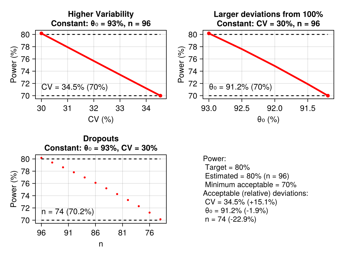
The computation carried out by power_analysis encompasses samplesize. This is evident in the graphical output above where the determination of n = 96 subjects is presented. A key computation is to consider the effect of miss-specification of the parameters as well as dropouts (subjects leaving the experiment without completion) affect power. For this power_analysis varies peθ₀, CV, and the sample size n. The variation range is determined by min_power. This is an implicit argument to the function set at a default value of 0.7. It signifies the minimal acceptable power we can consider. Specifically, the parameters are varied until the point where the power drops below min_power.
In this example experimental design and study type power is monotonic in peθ₀, CV, and n. However, other cases exhibit non-monotonic behavior at some region. In any case, increasing of CV generally reduces power, decreasing of n (dropouts) reduces power, and for peθ₀, movement away from 1, reduces power.
BioequivalencePower.PowerAnalysisConstants — Type
PowerAnalysisConstants(min_power::Float64 = 0.7,
                       CV_step::Float64 = 0.005,
                       θ₀_step::Float64 = 0.005,
                       CV_reduction_factor = 2/3,
                       min_n::Int = 12,
                       do_plot::Bool = true)
This struct contains some arguments used for the power_analysis function.
Arguments
- 'min_power': The minimal level of acceptable power. Power analysis is carried down to this level of power.
- 'CV_step': The increments of the CV when scanning the CV.
- 'θ₀_step': The increments of the θ₀ when scanning θ₀.
- 'CVreductionfactor': When computing the CV, we start at the given CV multiplied by this reduction factor. This is important for cases where power is not monotone in the CV.
- 'min_n': Samples smaller than this value are not allowed.
- 'do_plot': Plot the results (default is
true). Otherwise only present textual output.
Adjusting α
The non-standard nature of some procedures, and in particular reference scaling and/or expanding limits studies, implies that in certain cases the type I error of the test exceeds the specified $\alpha$. This potentially increases consumer risk. The adjusted_α function exposes such cases, and in case type I error exceeds $\alpha$, it suggests a reduced (adjusted) $\alpha$ that yields the desired type I error. Here is an example:
result =
    adjusted_α(ExpandingLimitsRatioTOST, ED2x2x4ReplicateCrossover, CV = 0.35, peθ₀ = 0.92)
println("With fixed α: ", result.before_adjustment)
println("After adjustment: ", result.after_adjustment)
With fixed α: (α = 0.05, type_I_error = 0.06588999999999955, achieved_power = 0.8124699999999987, n = [13, 13])
After adjustment: (α = 0.03688847325257455, type_I_error = 0.04999999999999959, achieved_power = 0.7737100000000101, n = [13, 13])As is evident, in this case, when using the basic $\alpha = 0.05$ setting, and under other the assumptions CV = 0.35, peθ₀ = 0.82, the Type I error is about 6.58%. The function also determines the sample size set at 26 subject (13 per sequence). The adjustment determined by the function is then to set $\alpha = 0.03693$ and this corrects the setup so that the Type I error is at the desired 5%. However, in this case the adjusted $\alpha$ changes the power to about 77.4% when keeping the same sample size.
An extension is to then use the adjusted_α_with_samplesize function:
result = adjusted_α_with_samplesize(
    ExpandingLimitsRatioTOST,
    ED2x2x4ReplicateCrossover,
    CV = 0.35,
    peθ₀ = 0.92,
)
println("With fixed α: ", result.before_adjustment)
println("After adjustment: ", result.after_adjustment)
[ Info: Basic adjusted α has n_vector = [13, 13] with power = 0.7737100000000101 and adjusted α = 0.03688847325257455
[ Info: new n_vector = [14, 14] with power = 0.7986800000000012 and adjusted α = 0.036450661558256436
[ Info: new n_vector = [15, 15] with power = 0.8218100000000048 and adjusted α = 0.03634602431422124
With fixed α: (α = 0.05, type_I_error = 0.06660000000000094, achieved_power = 0.8565300000000039, n = [15, 15])
After adjustment: (α = 0.03634602431422124, type_I_error = 0.0500000000000002, achieved_power = 0.8218100000000048, n = [15, 15])This output of this function is verbose as it indicates the steps in searching for the sample size. It begins with the original sample size of 26 (13 per sequence) and then increases the sample size sequentially, each time adjusting $\alpha$ and considering the power. The function then stops when the target power (default is 80%) is achieved. The result is then to adjust $\alpha$ to about 0.03635 and set the sample size at 30 subjects (15 per sequence group).
Regulatory constants
Some study types, in particular reference scaling and/or expanding limits study types, behave differently based on the regulator. For this we can use the RegulatoryConstants type which encompasses related information about the regulator.
BioequivalencePower.RegulatoryConstants — Type
RegulatoryConstants(agency::Symbol = :user,
                    r_const::Float64,
                    cv_switch::Float64 = 0.3,
                    cv_cap::Float64,
                    apply_pe_constraints::Bool = true,
                    estimation_method::Symbol = :anova)
An object that holds a few constants of a regulator.
Arguments
agency: One of:fda,:ema,:hc,:gcc, or:user.r_const: The so-called "regulatory constant".cv_switch: CV threshold for switching to widened acceptance limits (switch above this threshold.)cv_cap: Maximal CV for widening acceptance limits (beyond this CV level is constant).apply_pe_constraints: Indicates if point estimate constraints should be applied (true).estimation_method: Either:anovaor:isc(inter-subject contrasts).
The supported in-built regulators are determined by Symbols:
:fda- Federal Drug Administration (FDA):ema- European Medicines Agency (EMA):hc- Health Canada (HC):gcc- Gulf Cooperation Council (GCC):user- A user specified set of constants not matching one of the above.
You can construct a set of regulatory constants based on one of the above symbols. For example for the FDA:
RegulatoryConstants(:fda)RegulatoryConstants
agency: Symbol fda
r_const: Float64 0.8925742052568391
cv_switch: Float64 0.3
cv_cap: Float64 Inf
apply_pe_constraints: Bool true
estimation_method: Symbol isc
or for the EMA:
RegulatoryConstants(:ema)RegulatoryConstants
agency: Symbol ema
r_const: Float64 0.76
cv_switch: Float64 0.3
cv_cap: Float64 0.5
apply_pe_constraints: Bool true
estimation_method: Symbol anova
The meaning of the fields r_const, cv_switch, cv_cap, apply_pe_constraints, and estimation_method are described in the reference scaling and/or expanding limits section.
For a :user set of constants, either to be used for other agencies or for experimentation, use syntax such as:
RegulatoryConstants(r_const = 0.9, cv_cap = 0.6)RegulatoryConstants
agency: Symbol user
r_const: Float64 0.9
cv_switch: Float64 0.3
cv_cap: Float64 0.6
apply_pe_constraints: Bool true
estimation_method: Symbol anova
Note that the values of cv_switch, apply_pe_constraints, and estimation_method have default values, yet these may be changed as well.
Tables of designs and supported features
In general, you can see the supported features by invoking the supported_designs_and_studies function which returns a NamedTuple with keys :designs, :studies, :legend, and :methods. The values of the NamedTuple are DataFrames that summarize the available functionality.
For example, this output summarizes which methods are implemented for the core functions of the package, mapping study types, and functionality:
supported_designs_and_studies()[:methods]| Row | StudyType | power | samplesize | pvalue | confint | adjusted_α | adjusted_α_with_samplesize | power_analysis |
|---|---|---|---|---|---|---|---|---|
| Any | String | String | String | String | String | String | String | |
| 1 | DifferenceTOST | yes | yes | yes | yes | |||
| 2 | RatioTOST | yes | yes | yes | yes | yes | ||
| 3 | TwoDifferenceTOSTs | yes | yes | |||||
| 4 | TwoRatioTOSTs | yes | yes | |||||
| 5 | FiducialRatioTOST | yes | yes | yes | ||||
| 6 | NonInferiorityDifferenceOST | yes | yes | |||||
| 7 | NonInferiorityRatioOST | yes | yes | |||||
| 8 | ExpandingLimitsRatioTOST | yes | yes | yes | yes | yes | ||
| 9 | ReferenceScaledRatioTOST | yes | yes | yes | yes | |||
| 10 | NarrowTherapeuticIndexDrugRatioTOST | yes | yes | yes | ||||
| 11 | DoseProportionalityStudy | yes | yes | |||||
| 12 | (BayesianWrapper, DifferenceTOST) | yes | yes | |||||
| 13 | (BayesianWrapper, RatioTOST) | yes | yes | |||||
| 14 | (BayesianWrapper, NonInferiorityDifferenceOST) | yes | yes | |||||
| 15 | (BayesianWrapper, NonInferiorityRatioOST) | yes | yes |
As is evident power and samplesize are implemented for all study types, yet other functions are only implemented for specific study types.
This output is a table with some details about designs:
supported_designs_and_studies()[:designs]| Row | DesignType | DesignString | NumTreatments | NumSequences | NumPeriods | VarianceScalingConstant | DegreesOfFreedom | RobustDegreesOfFreedom |
|---|---|---|---|---|---|---|---|---|
| DataType | String | Union… | Union… | Union… | Union… | String | String | |
| 1 | ED2Parallel | parallel | 2 | 2 | 1 | 1.0 | n - 2 | n - 2 |
| 2 | ED2x2Crossover | 2x2 | 2 | 2 | 2 | 0.5 | n - 2 | n - 2 |
| 3 | ED3x3Crossover | 3x3 | 3 | 3 | 3 | 0.222222 | 2n - 4 | n - 3 |
| 4 | ED3x6x3Crossover | 3x6x3 | 3 | 6 | 3 | 0.0555556 | 2n - 4 | n - 6 |
| 5 | ED4x4Crossover | 4x4 | 4 | 4 | 4 | 0.125 | 3n - 6 | n - 4 |
| 6 | ED2x2x3ReplicateCrossover | 2x2x3 | 2 | 2 | 3 | 0.375 | 2n - 3 | n - 2 |
| 7 | ED2x2x4ReplicateCrossover | 2x2x4 | 2 | 2 | 4 | 0.25 | 3n - 4 | n - 2 |
| 8 | ED2x4x4ReplicateCrossover | 2x4x4 | 2 | 4 | 4 | 0.0625 | 3n - 4 | n - 4 |
| 9 | ED2x3x3PartialReplicate | 2x3x3 | 2 | 3 | 3 | 0.166667 | 2n - 3 | n - 3 |
| 10 | ED2x4x2Balaam | 2x4x2 | 2 | 4 | 2 | 0.5 | n - 2 | n - 2 |
| 11 | ED2x2x2RepeatedCrossover | 2x2x2r | 2 | 2 | 2 | 0.25 | 3n - 2 | n - 2 |
| 12 | EDPaired | paired | 1 | 1 | 1 | 2.0 | n - 1 | n - 1 |
| 13 | EDGeneralCrossover | A general design used for dose prop: EDGeneralCrossover | - | - | ||||
| 14 | EDGeneralParallel | A general design used for dose prop: EDGeneralParallel | - | - | ||||
| 15 | EDGeneral | A general design used for dose prop: EDGeneral | - | - |
Now different study-design combinations are possible and in each case power can be computed using a specific algorithm. This large table outlines all the study-design combinations
supported_designs_and_studies()[:studies]| Row | StudyType | ED2Parallel | ED2x2Crossover | ED3x3Crossover | ED3x6x3Crossover | ED4x4Crossover | ED2x2x3ReplicateCrossover | ED2x2x4ReplicateCrossover | ED2x4x4ReplicateCrossover | ED2x3x3PartialReplicate | ED2x4x2Balaam | ED2x2x2RepeatedCrossover | EDPaired | EDGeneralCrossover | EDGeneralParallel | EDGeneral |
|---|---|---|---|---|---|---|---|---|---|---|---|---|---|---|---|---|
| Any | String | String | String | String | String | String | String | String | String | String | String | String | String | String | String | |
| 1 | DifferenceTOST | num|mc | num|mc | num|mc | num|mc | num|mc | num|mc | num|mc | num|mc | num|mc | num|mc | num|mc | num|mc | - | - | - |
| 2 | RatioTOST | num|mc | num|mc|slmc | num|mc | num|mc | num|mc | num|mc|slmc | num|mc|slmc | num|mc | num|mc|slmc | num|mc | num|mc | num|mc | _ | _ | _ |
| 3 | TwoDifferenceTOSTs | mc | mc | mc | mc | mc | mc | mc | mc | mc | mc | mc | mc | _ | _ | _ |
| 4 | TwoRatioTOSTs | mc | mc | mc | mc | mc | mc | mc | mc | mc | mc | mc | mc | _ | _ | _ |
| 5 | FiducialRatioTOST | mc | mc | - | - | - | - | - | - | - | - | - | - | _ | _ | _ |
| 6 | NonInferiorityDifferenceOST | num | num | num | num | num | num | num | num | num | num | num | num | _ | _ | _ |
| 7 | NonInferiorityRatioOST | num | num | num | num | num | num | num | num | num | num | num | num | _ | _ | _ |
| 8 | ExpandingLimitsRatioTOST | - | - | - | - | - | mc|slmc | mc|slmc | - | mc|slmc | - | - | - | _ | _ | _ |
| 9 | ReferenceScaledRatioTOST | - | - | - | - | - | mc|slmc | mc|slmc | - | mc|slmc | - | - | - | _ | _ | _ |
| 10 | NarrowTherapeuticIndexDrugRatioTOST | - | - | - | - | - | mc | mc | - | - | - | - | - | _ | _ | _ |
| 11 | DoseProportionalityStudy | - | - | - | - | - | - | - | - | - | - | - | - | anum | anum | anum |
| 12 | (BayesianWrapper, DifferenceTOST) | nume | nume | nume | nume | nume | nume | nume | nume | nume | nume | nume | nume | _ | _ | _ |
| 13 | (BayesianWrapper, RatioTOST) | nume | nume | nume | nume | nume | nume | nume | nume | nume | nume | nume | nume | _ | _ | _ |
| 14 | (BayesianWrapper, NonInferiorityDifferenceOST) | nume | nume | nume | nume | nume | nume | nume | nume | nume | nume | nume | nume | _ | _ | _ |
| 15 | (BayesianWrapper, NonInferiorityRatioOST) | nume | nume | nume | nume | nume | nume | nume | nume | nume | nume | nume | nume | _ | _ | _ |
The legend for the type of power computation is here:
supported_designs_and_studies()[:legend]| Row | Code | Meaning |
|---|---|---|
| String | String | |
| 1 | num | Numerical |
| 2 | anum | Approximate Numerical |
| 3 | nume | Numerical Expectation |
| 4 | mc | Monte Carlo |
| 5 | slmc | Subject Level Monte Carlo |
Bibliography and further reading
General texts supporting bioequivalence analysis include:
- [18]
- S. D. Patterson and B. Jones. Bioequivalence and statistics in clinical pharmacology (CRC Press, 2017).
- [19]
- S.-C. Chow and J.-P. Liu. Design and analysis of bioavailability and bioequivalence studies (CRC Press, 2008).
- [20]
- X. Y. Lawrence and B. V. Li. FDA bioequivalence standards. Vol. 13 (Springer, 2014).