Parallel Study Design
The Getting started example assumes a crossover design where every subject receives both the IV reference and the oral test formulations. This guide demonstrates a parallel design where one group receives IV only and a separate group receives the oral formulations. Since oral subjects have no individual IV data, UIR fitting uses the mean_uir_fallback=true option to apply the mean UIR from the IV group.
Simulated data
Group A (subjects 1–10) receives only the IV bolus. Group B (subjects 11–20) receives three oral formulations but no IV data.
first(pk_df, 8)| Row | id | formulation | time | conc |
|---|---|---|---|---|
| Int64 | String | Float64 | Float64 | |
| 1 | 1 | IV | 0.0 | 8.84915 |
| 2 | 1 | IV | 0.5 | 7.86636 |
| 3 | 1 | IV | 1.0 | 6.99273 |
| 4 | 1 | IV | 1.5 | 6.21611 |
| 5 | 1 | IV | 2.0 | 5.52575 |
| 6 | 1 | IV | 2.5 | 4.91207 |
| 7 | 1 | IV | 3.0 | 4.36653 |
| 8 | 1 | IV | 3.5 | 3.88159 |
first(diss_df, 8)| Row | formulation | time | diss |
|---|---|---|---|
| String | Float64 | Float64 | |
| 1 | FormA | 0.0 | 0.0 |
| 2 | FormA | 0.5 | 0.0432318 |
| 3 | FormA | 1.0 | 0.117503 |
| 4 | FormA | 1.5 | 0.20518 |
| 5 | FormA | 2.0 | 0.297811 |
| 6 | FormA | 2.5 | 0.389884 |
| 7 | FormA | 3.0 | 0.477703 |
| 8 | FormA | 3.5 | 0.558902 |
Running the pipeline with mean_uir_fallback
The key parameter is mean_uir_fallback=true: oral subjects (who lack IV data) are deconvolved using the population-mean UIR computed from the IV-only group.
result = run_ivivc(
    pk_df,
    diss_df;
    fast_formulation = "IV",
    validation_formulation = "FormB",
    times = collect(range(0.0, 48.0, length = 101)),
    mean_uir_fallback = true,
);
UIR fits
Only the IV-group subjects have individual UIR fits. The mean UIR is applied to the oral-group subjects during deconvolution.
first(result.uir_df, 8)| Row | id | formulation | uir |
|---|---|---|---|
| Any | String | PolyExpo… | |
| 1 | 3 | IV | PolyExponential{Float64, Float64}([9.87871], [0.199118], 1.0, 1.0) |
| 2 | 2 | IV | PolyExponential{Float64, Float64}([10.0916], [0.183047], 1.0, 1.0) |
| 3 | 1 | IV | PolyExponential{Float64, Float64}([8.84915], [0.235451], 1.0, 1.0) |
| 4 | 4 | IV | PolyExponential{Float64, Float64}([12.5107], [0.198256], 1.0, 1.0) |
| 5 | 5 | IV | PolyExponential{Float64, Float64}([8.84737], [0.204248], 1.0, 1.0) |
| 6 | 6 | IV | PolyExponential{Float64, Float64}([8.72146], [0.230911], 1.0, 1.0) |
| 7 | 8 | IV | PolyExponential{Float64, Float64}([9.39545], [0.203476], 1.0, 1.0) |
| 8 | 7 | IV | PolyExponential{Float64, Float64}([9.70289], [0.192404], 1.0, 1.0) |
Model parameters
coeftable(result.model)| Row | parameter | constant | estimate |
|---|---|---|---|
| Symbol | Bool | Float64 | |
| 1 | abs_scale | false | 1.0482 |
| 2 | abs_intercept | false | 0.0101697 |
| 3 | time_scale | false | 0.793854 |
| 4 | time_shift | false | -0.170846 |
Plots
concentration_profiles(result)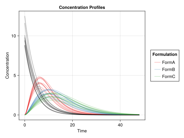
dissolution_profiles(result)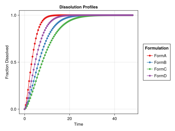
absorption_profiles(result)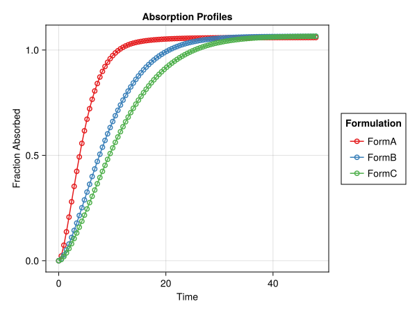
levy_plot(result)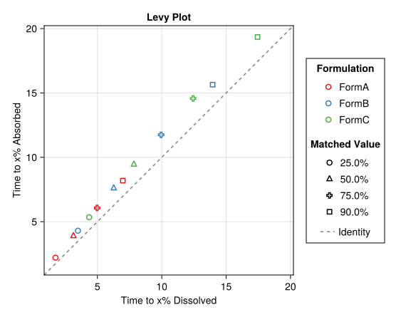
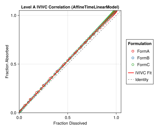
ivivc_correlation(result)