Mixture Models
PumasMixtureModel lives in the Pumas.Experimental module. The API is experimental and subject to change in future releases without deprecations.
A finite mixture model describes a population as a blend of a small number of subpopulations. Each subject belongs to exactly one subpopulation, but the membership is not observed, so the likelihood of a subject's data is averaged over the subpopulations with the mixture probabilities as weights. Typical use cases in pharmacometrics are
- a parameter whose random effect distribution is bimodal, for example the clearance of a drug metabolized by a polymorphic enzyme, where poor and extensive metabolizers form two subpopulations with distinct typical clearances,
- a population in which different subjects are best described by different structural models, for example responders and non-responders in a pharmacodynamic model, or subjects with and without a metabolic pathway.
In Pumas, a mixture model is built from ordinary @model definitions, one per subpopulation, with the PumasMixtureModel type.
Table of contents
Defining a mixture model
A PumasMixtureModel is constructed from a tuple of @model definitions, one per component, and a name for the mixture probability parameter:
using Pumas.Experimental: PumasMixtureModel

mix = PumasMixtureModel((model₁, model₂, ..., modelₖ), :mixprobs => SimplexDomain(K))
The marginal likelihood of a subject's observations $y$ is
\[L(y \mid \theta, \pi) = \sum_{k=1}^{K} \pi_k L_k(y \mid \theta_k)\]
where $L_k$ is the ordinary marginal likelihood of component $k$, that is, the likelihood of the @model with its random effects integrated out, $\theta_k$ is the subset of the parameters used by component $k$, and $\pi = (\pi_1, \ldots, \pi_K)$ are the mixture probabilities. The population likelihood is the product over subjects, so each subject is assigned to the components independently.
The components and the mixture probabilities are tied together by a few rules.
Parameters are shared by name. The parameter set of the mixture is the union of the parameter sets of the components. If two components both declare
tvcl, the same value is used in both. A parameter that should differ between the components therefore needs a distinct name in each component, for exampletvcl_poorandtvcl_extensive.Shared parameters must be declared identically. A parameter that appears in several components must use the same domain (or the same prior) in all of them, including the bounds and the initial value. The constructor throws an error otherwise.
The mixture probabilities are a parameter. They are added to the parameter set under the name given in the
Pair, constrained to the unit simplex, and estimated together with the other parameters. The name must not clash with a parameter of a component. The domain is eitherSimplexDomain(K), which only constrains the probabilities to be non-negative and sum to one, with the uniform vectorfill(1/K, K)as the initial value, orDirichlet(K, α)orDirichlet(α)from Distributions.jl, whose mean is used as the initial value. None of the supported estimation methods uses priors, so the Dirichlet distribution currently has no other effect.
At least two components are required, and the length of the simplex must match the number of components.
The components need not share their dynamics, random effects or error model. They must, however, model the same observed variables, since the likelihoods of the components are evaluated on the same data.
Starting values
If the components have the same structure and differ only in their component-specific parameters, as in the first example below, the likelihood is invariant to permuting their labels. If all component-specific parameters start at the same values, the components are indistinguishable at the starting point and the optimizer has no direction in which to separate them. Always start the component-specific parameters at distinct values that reflect the hypothesized subpopulations. The same symmetry means that a refit from different starting values, or the refits in a Bootstrap or SIR inference, may return the components in a different order (label switching). Component-specific parameters and the mixture probabilities should be read with that in mind.
Example 1: A mixture in the random effects
The first example describes a drug whose clearance is bimodal because it is metabolized by a polymorphic enzyme. A subject is either a poor or an extensive metabolizer. Within each subpopulation, the clearance is log-normally distributed around the typical value of that subpopulation, with the same between-subject variability in both. In other words, the logarithm of the individual clearance follows a mixture of two normal distributions with different means and a common variance.
In Pumas, this is expressed as two components that are identical except for the name of the typical clearance. Everything else, that is, the absorption rate, the volume, the random effect covariance Ω and the residual error, is shared by using the same parameter names in both components.
using Pumas
using Pumas.Experimental: PumasMixtureModel, responsibilities, subpopulation, icl
using PumasUtilities
using DataFrames
using DataFramesMeta
using SummaryTables
using Random
using CairoMakie
using AlgebraOfGraphics

pk_poor = @model begin
    @param begin
        tvka ∈ RealDomain(lower = 0.0)
        tvcl_poor ∈ RealDomain(lower = 0.0)
        tvvc ∈ RealDomain(lower = 0.0)
        Ω ∈ PDiagDomain(3)
        σ_prop ∈ RealDomain(lower = 0.0)
    end
    @random begin
        η ~ MvNormal(Ω)
    end
    @pre begin
        Ka = tvka * exp(η[1])
        CL = tvcl_poor * exp(η[2])
        Vc = tvvc * exp(η[3])
    end
    @dynamics Depots1Central1
    @derived begin
        cp := @. Central / Vc
        dv ~ @. ProportionalNormal(cp, σ_prop)
    end
end

pk_extensive = @model begin
    @param begin
        tvka ∈ RealDomain(lower = 0.0)
        tvcl_extensive ∈ RealDomain(lower = 0.0)
        tvvc ∈ RealDomain(lower = 0.0)
        Ω ∈ PDiagDomain(3)
        σ_prop ∈ RealDomain(lower = 0.0)
    end
    @random begin
        η ~ MvNormal(Ω)
    end
    @pre begin
        Ka = tvka * exp(η[1])
        CL = tvcl_extensive * exp(η[2])
        Vc = tvvc * exp(η[3])
    end
    @dynamics Depots1Central1
    @derived begin
        cp := @. Central / Vc
        dv ~ @. ProportionalNormal(cp, σ_prop)
    end
end

mix_cl = PumasMixtureModel((pk_poor, pk_extensive), :mixprobs => SimplexDomain(2))
PumasMixtureModel
Number of components: 2
Parameters: (:tvka, :tvcl_poor, :tvvc, :Ω, :σ_prop, :tvcl_extensive, :mixprobs)The parameter set of the mixture is the union of the two parameter sets plus the mixture probabilities:
init_params(mix_cl)(tvka = 1.0, tvcl_poor = 1.0, tvvc = 1.0, Ω = [1.0 0.0 0.0; 0.0 1.0 0.0; 0.0 0.0 1.0], σ_prop = 1.0, tvcl_extensive = 1.0, mixprobs = [0.5, 0.5])Simulating from a mixture model
To have data to fit, we simulate a population of 60 subjects after a single oral dose, 18 poor and 42 extensive metabolizers. The membership is recorded as the covariate metabolizer of each subject. The covariate is not used by the models, it is only carried along into the data frames and plots below so that the classification can be checked against the truth later in this example:
true_param_cl = (;
    tvka = 1.0,
    tvcl_poor = 1.0,
    tvcl_extensive = 4.0,
    tvvc = 30.0,
    Ω = Diagonal([0.09, 0.09, 0.09]),
    σ_prop = 0.2,
    mixprobs = [0.3, 0.7],
)

labels_cl = ["poor", "extensive"]
true_subpopulation = vcat(fill(1, 18), fill(2, 42))
dose = DosageRegimen(100; time = 0)
obstimes = [0.5, 1.0, 2.0, 4.0, 8.0, 12.0, 24.0]
skeleton_cl = [
    Subject(;
        id = i,
        events = dose,
        time = obstimes,
        covariates = (; metabolizer = labels_cl[k]),
    ) for (i, k) in enumerate(true_subpopulation)
]
simobs accepts a PumasMixtureModel and draws, for every subject, the component from the mixture probabilities before simulating from that component:
Random.seed!(1)
simobs(mix_cl, skeleton_cl, true_param_cl)
Simulated population (Vector{<:Subject})
Simulated subjects: 60
Simulated variables: dvThe simulated observations do not record which component each subject was drawn from, and the draw ignores the metabolizer covariate. To obtain a population whose membership is known, we instead simulate each subpopulation from its own component:
sims_poor = simobs(
    pk_poor,
    skeleton_cl[true_subpopulation.==1],
    true_param_cl[(:tvka, :tvcl_poor, :tvvc, :Ω, :σ_prop)],
)
sims_extensive = simobs(
    pk_extensive,
    skeleton_cl[true_subpopulation.==2],
    true_param_cl[(:tvka, :tvcl_extensive, :tvvc, :Ω, :σ_prop)],
)
pop_cl = Subject.(vcat(sims_poor, sims_extensive))
The two subpopulations are visible in the simulated concentration-time profiles. The poor metabolizers eliminate the drug slowly and still have a high concentration at 24 hours, while the extensive metabolizers show a steeper decline:
df_pop_cl = DataFrame(pop_cl; include_events = false)

plt_cl =
    data(df_pop_cl) *
    mapping(
        :time => "Time (h)",
        :dv => "Concentration";
        color = :metabolizer => sorter(labels_cl) => "Metabolizer",
        group = :id,
    ) *
    visual(Lines; alpha = 0.6)
draw(plt_cl; axis = (; yscale = log10))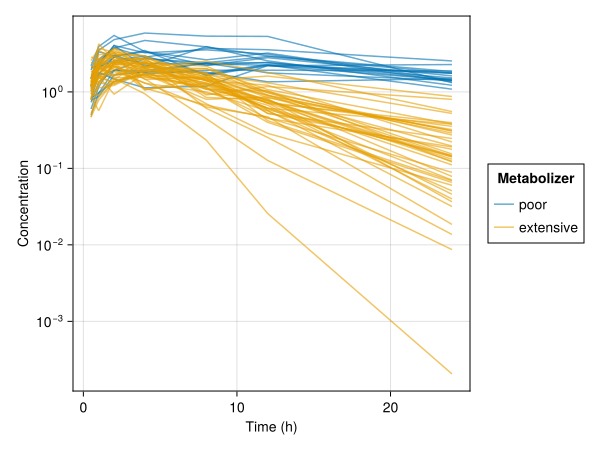
Fitting a mixture model
A mixture model is fitted with fit like a regular Pumas model. The supported likelihood approximations are FOCE, LaplaceI, FO and NaivePooled, with the usual keyword arguments constantcoef, optim_alg, optim_options, diffeq_options and ensemblealg. As discussed above, the two typical clearances are started at distinct values:
init_cl = (;
    tvka = 1.0,
    tvcl_poor = 2.0,
    tvcl_extensive = 3.0,
    tvvc = 30.0,
    Ω = Diagonal([0.1, 0.1, 0.1]),
    σ_prop = 0.2,
    mixprobs = [0.5, 0.5],
)

fit_cl = fit(mix_cl, pop_cl, init_cl, FOCE(); optim_options = (; show_trace = false))
FittedPumasMixtureModel
Mixture model components: 2
Number of subjects: 60
Observation records: Active Missing
dv: 420 0
Total: 420 0
Number of parameters: Constant Optimized
0 9
Likelihood approximation: FOCE
Likelihood optimizer: BFGS
Termination Reason: GradientNorm
Log-likelihood value: -245.99851
---------------------------
Estimate
---------------------------
tvka 0.97621
tvcl_poor 0.89613
tvvc 31.519
Ω₁,₁ 0.086545
Ω₂,₂ 0.079983
Ω₃,₃ 0.082808
σ_prop 0.22018
tvcl_extensive 4.2526
mixprobs₁ 0.31892
mixprobs₂ 0.68108
---------------------------The two typical clearances have separated, and the estimated mixture probabilities are close to the fractions of poor and extensive metabolizers in the simulated population. The usual accessors, coef, coeftable, loglikelihood, aic and bic, are available. The degrees of freedom count the mixture probabilities as $K - 1$ free parameters.
Inference
infer computes asymptotic standard errors from the observed information of the mixture likelihood, by default with the sandwich estimator. The standard errors and confidence intervals of the mixture probabilities are reported on the probability scale:
infer_cl = infer(fit_cl)Asymptotic inference results using sandwich estimator
Mixture model components: 2
Number of subjects: 60
Observation records: Active Missing
dv: 420 0
Total: 420 0
Number of parameters: Constant Optimized
0 9
Likelihood approximation: FOCE
Likelihood optimizer: BFGS
Termination Reason: GradientNorm
Log-likelihood value: -245.99851
---------------------------------------------------------------
Estimate SE 95.0% C.I.
---------------------------------------------------------------
tvka 0.97621 0.057006 [ 0.86449 ; 1.0879 ]
tvcl_poor 0.89613 0.083585 [ 0.73231 ; 1.06 ]
tvvc 31.519 1.3886 [ 28.797 ; 34.24 ]
Ω₁,₁ 0.086545 0.037257 [ 0.013523; 0.15957]
Ω₂,₂ 0.079983 0.028063 [ 0.024982; 0.13499]
Ω₃,₃ 0.082808 0.016369 [ 0.050725; 0.11489]
σ_prop 0.22018 0.010237 [ 0.20012 ; 0.24025]
tvcl_extensive 4.2526 0.2078 [ 3.8454 ; 4.6599 ]
mixprobs₁ 0.31892 0.061954 [ 0.19749 ; 0.44034]
mixprobs₂ 0.68108 0.061954 [ 0.55966 ; 0.80251]
---------------------------------------------------------------infer with Bootstrap and SIR is also supported. The bootstrap refits each resampled population with the optimizer settings of the original fit. Since the components can be relabeled between refits, see Starting values, the summaries of component-specific parameters from these methods should be interpreted with care.
Classifying the subjects
Once the mixture has been fitted, each subject can be classified. The posterior probability that subject $i$ belongs to component $k$ given its data, often called the responsibility of component $k$ for subject $i$, is
\[w_{ik} = \frac{\pi_k L_k(y_i \mid \theta_k)}{\sum_j \pi_j L_j(y_i \mid \theta_j)}\]
responsibilities returns one probability vector per subject:
w_cl = responsibilities(fit_cl)
first(w_cl, 5)
5-element Vector{Vector{Float64}}:
[0.9992411905650332, 0.00075880943496684]
[0.9999782369162998, 2.1763083700267063e-5]
[0.9998650519948985, 0.0001349480051014613]
[0.999998826820725, 1.1731792748313565e-6]
[0.999920756192937, 7.924380706292253e-5]subpopulation returns the most probable component of each subject. In this example, we know the true membership, so we can calculate the fraction of correctly classified subjects:
mean(subpopulation(fit_cl) .== true_subpopulation)0.9833333333333333At the maximum likelihood estimate, the average responsibility of a component equals its estimated mixture probability, up to the convergence tolerance of the optimizer:
mean(w_cl)2-element Vector{Float64}:
0.31891550603763813
0.681084493962362Choosing the number of components
The number of components is usually chosen by comparing the fits with $1, 2, \ldots$ components. The log-likelihood, aic and bic are available for that purpose, but the usual likelihood ratio test does not apply when comparing a mixture with a model with one component less: the smaller model lies on the boundary of the parameter space of the larger one, and the parameters of the removed component are not identifiable under the smaller model. In addition to bic, icl computes the integrated completed likelihood [3], which adds a penalty for the uncertainty in the classification of the subjects. The ICL is at least as large as the BIC and favors mixtures with well separated components. Lower is better. A model with a single component classifies every subject with certainty, so its ICL equals its BIC. Both criteria favor the mixture over a single-component model here:
fit_single = fit(
    pk_extensive,
    pop_cl,
    init_cl[(:tvka, :tvcl_extensive, :tvvc, :Ω, :σ_prop)],
    FOCE();
    optim_options = (; show_trace = false),
)
comparison_cl = DataFrame(;
    model = ["one component", "two components"],
    bic = [bic(fit_single), bic(fit_cl)],
    icl = [bic(fit_single), icl(fit_cl)],
)
simple_table(comparison_cl, [:model => "Model", :bic => "BIC", :icl => "ICL"])| Model | BIC | ICL |
| one component | 568 | 568 |
| two components | 546 | 548 |
Diagnostics
inspect collects the predictions, weighted residuals, empirical Bayes estimates, individual coefficients and dose control parameters of a fitted mixture model. These are computed per component, so, for example, predict and empirical_bayes return a tuple with one entry per component for each subject:
empirical_bayes(fit_cl)[1]((η = [-0.1247735162380162, 0.002380615224743835, 0.4712626505692884],), (η = [-0.2566489887810848, -0.9492162616979872, 0.3565625575768908],))The NPDE and EWRES are simulation based and are computed from the marginal predictive distribution of the mixture, which samples the component along with the random effects and the residual error. They are therefore defined for the mixture as a whole, not per component, and are available by passing a positive nsim to inspect:
inspect_cl = inspect(fit_cl; nsim = 100)FittedPumasMixtureModelInspection
Number of components: 2
Mixture probabilities: [0.3189156038474721, 0.6810843961525278]
Likelihood approximation used for weighted residuals: FOCEThe DataFrame of the inspection has one row per observation and dose record. The population quantities dv_pred and dv_wres are averaged over the components with the mixture probabilities as weights, while the individual quantities dv_ipred and dv_iwres, the random effects, the individual coefficients and the dynamic variables are taken from the most probable component of each subject. The responsibilities are included as the columns probability₁, probability₂, …, and the most probable component as subpopulation:
df_cl = DataFrame(inspect_cl)
@chain df_cl begin
    @rsubset :evid == 0
    @select :id :time :dv :dv_pred :dv_ipred :dv_npde :metabolizer :probability₁ :probability₂ :subpopulation
    first(7)
    simple_table
end| id | time | dv | dv_pred | dv_ipred | dv_npde | metabolizer | probability₁ | probability₂ | subpopulation |
| 1 | 0.5 | 0.776 | 1.19 | 0.69 | -0.994 | poor | 0.999 | 0.000759 | 1 |
| 1 | 1 | 0.874 | 1.87 | 1.13 | -1.28 | poor | 0.999 | 0.000759 | 1 |
| 1 | 2 | 1.66 | 2.4 | 1.59 | 0.228 | poor | 0.999 | 0.000759 | 1 |
| 1 | 4 | 1.83 | 2.32 | 1.82 | 0.228 | poor | 0.999 | 0.000759 | 1 |
| 1 | 8 | 1.81 | 1.68 | 1.75 | 0.878 | poor | 0.999 | 0.000759 | 1 |
| 1 | 12 | 1.35 | 1.24 | 1.63 | 0 | poor | 0.999 | 0.000759 | 1 |
| 1 | 24 | 1.49 | 0.625 | 1.32 | 1.64 | poor | 0.999 | 0.000759 | 1 |
The individual clearances of the inspection make the mixture visible. A histogram of the individual clearances, colored by the assigned component, shows the two subpopulations:
per_subject = @chain df_cl begin
    @select :id :metabolizer :CL :probability₁ :subpopulation
    unique
end

plt_hist =
    data(per_subject) *
    mapping(
        :CL => "Individual clearance";
        color = :subpopulation => renamer(labels_cl) => "Assigned component",
    ) *
    histogram(; bins = 0:0.5:12)
draw(plt_hist)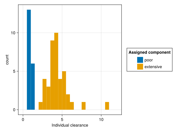
Plotting the responsibilities against the individual clearances shows how confident the classification of each subject is. Only a few subjects with a clearance between the two typical values have a responsibility away from zero or one:
plt_prob =
    data(per_subject) *
    mapping(
        :CL => "Individual clearance",
        :probability₁ => "Probability of the poor metabolizer component";
        color = :subpopulation => renamer(labels_cl) => "Assigned component",
    ) *
    visual(Scatter)
draw(plt_prob)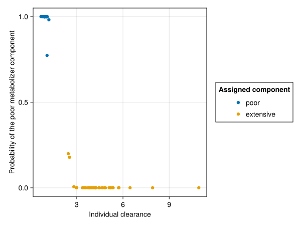
The inspection of a fitted mixture model can be passed to the goodness-of-fit plots of PumasPlots, and the subpopulation column can be used to stratify them by the assigned component. For example, with observations_vs_ipredictions:
observations_vs_ipredictions(inspect_cl; stratify_by = :subpopulation)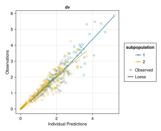
The η- and ϵ-shrinkage are reported per component by ηshrinkage and ϵshrinkage. Note that each component's shrinkage is computed from the empirical Bayes estimates of all subjects under that component, including the subjects that belong to the other components. findinfluential ranks the subjects by their marginal mixture log-likelihood.
Example 2: A mixture of two dynamical systems
The components of a mixture model do not have to share their dynamics. A common application is a pharmacodynamic analysis in which some subjects do not respond to the drug at all. In the second example, the drug lowers a biomarker by inhibiting its production in the responders, whereas the biomarker of the non-responders is unaffected by the drug and only fluctuates around its baseline. Both components share a one-compartment pharmacokinetic model and the turnover of the biomarker, including the random effects and the residual error models. The inhibitory drug effect, with the parameters tvimax and tvic50, only exists in the responder component.
using Pumas
using Pumas.Experimental: PumasMixtureModel, responsibilities, subpopulation, icl
using DataFrames
using DataFramesMeta
using SummaryTables
using Random
using CairoMakie
using AlgebraOfGraphics

nonresponder = @model begin
    @param begin
        tvka ∈ RealDomain(lower = 0.0)
        tvcl ∈ RealDomain(lower = 0.0)
        tvvc ∈ RealDomain(lower = 0.0)
        tvr0 ∈ RealDomain(lower = 0.0)
        tvkout ∈ RealDomain(lower = 0.0)
        Ω ∈ PDiagDomain(3)
        σ_pk ∈ RealDomain(lower = 0.0)
        σ_pd ∈ RealDomain(lower = 0.0)
    end
    @random begin
        η ~ MvNormal(Ω)
    end
    @pre begin
        Ka = tvka * exp(η[1])
        CL = tvcl * exp(η[2])
        Vc = tvvc
        R0 = tvr0 * exp(η[3])
        kout = tvkout
        kin = R0 * kout
    end
    @init begin
        Response = R0
    end
    @dynamics begin
        Depot' = -Ka * Depot
        Central' = Ka * Depot - CL / Vc * Central
        Response' = kin - kout * Response
    end
    @derived begin
        cp := @. Central / Vc
        conc ~ @. ProportionalNormal(cp, σ_pk)
        resp ~ @. Normal(Response, σ_pd)
    end
end

responder = @model begin
    @param begin
        tvka ∈ RealDomain(lower = 0.0)
        tvcl ∈ RealDomain(lower = 0.0)
        tvvc ∈ RealDomain(lower = 0.0)
        tvr0 ∈ RealDomain(lower = 0.0)
        tvkout ∈ RealDomain(lower = 0.0)
        tvimax ∈ RealDomain(lower = 0.0, upper = 1.0)
        tvic50 ∈ RealDomain(lower = 0.0)
        Ω ∈ PDiagDomain(3)
        σ_pk ∈ RealDomain(lower = 0.0)
        σ_pd ∈ RealDomain(lower = 0.0)
    end
    @random begin
        η ~ MvNormal(Ω)
    end
    @pre begin
        Ka = tvka * exp(η[1])
        CL = tvcl * exp(η[2])
        Vc = tvvc
        R0 = tvr0 * exp(η[3])
        kout = tvkout
        kin = R0 * kout
        Imax = tvimax
        IC50 = tvic50
    end
    @init begin
        Response = R0
    end
    @dynamics begin
        Depot' = -Ka * Depot
        Central' = Ka * Depot - CL / Vc * Central
        Response' = kin * (1 - Imax * Central / (IC50 * Vc + Central)) - kout * Response
    end
    @derived begin
        cp := @. Central / Vc
        conc ~ @. ProportionalNormal(cp, σ_pk)
        resp ~ @. Normal(Response, σ_pd)
    end
end

mix_pd = PumasMixtureModel((nonresponder, responder), :mixprobs => SimplexDomain(2))
PumasMixtureModel
Number of components: 2
Parameters: (:tvka, :tvcl, :tvvc, :tvr0, :tvkout, :Ω, :σ_pk, :σ_pd, :tvimax, :tvic50, :mixprobs)The dynamic variables of the mixture are the union of the dynamic variables of the components. Here, the components define the same three states, but the components could also have different numbers of compartments.
dynamics_names(mix_pd)3-element Vector{String}:
"Depot"
"Central"
"Response"We simulate 15 non-responders and 35 responders who receive a daily dose for a week. The drug concentration and the biomarker are sampled at the same times, densely on the first day and once per day thereafter. As in the first example, the true membership is recorded as a covariate, here named status:
true_param_pd = (;
    tvka = 1.0,
    tvcl = 3.0,
    tvvc = 30.0,
    tvr0 = 100.0,
    tvkout = 0.1,
    tvimax = 0.8,
    tvic50 = 1.0,
    Ω = Diagonal([0.09, 0.09, 0.04]),
    σ_pk = 0.15,
    σ_pd = 5.0,
    mixprobs = [0.3, 0.7],
)

labels_pd = ["non-responder", "responder"]
true_subpopulation_pd = vcat(fill(1, 15), fill(2, 35))
doses = DosageRegimen(100; time = 0, ii = 24, addl = 6)
obstimes_pd = [0.5, 1.0, 2.0, 4.0, 8.0, 12.0, 24.0, 48.0, 72.0, 96.0, 120.0, 144.0, 168.0]
skeleton_pd = [
    Subject(;
        id = i,
        events = doses,
        time = obstimes_pd,
        covariates = (; status = labels_pd[k]),
    ) for (i, k) in enumerate(true_subpopulation_pd)
]

Random.seed!(3)
sims_non = simobs(
    nonresponder,
    skeleton_pd[true_subpopulation_pd.==1],
    true_param_pd[(:tvka, :tvcl, :tvvc, :tvr0, :tvkout, :Ω, :σ_pk, :σ_pd)],
)
sims_resp = simobs(
    responder,
    skeleton_pd[true_subpopulation_pd.==2],
    true_param_pd[(
        :tvka,
        :tvcl,
        :tvvc,
        :tvr0,
        :tvkout,
        :tvimax,
        :tvic50,
        :Ω,
        :σ_pk,
        :σ_pd,
    )],
)
pop_pd = Subject.(vcat(sims_non, sims_resp))
The biomarker of the responders drops during the first day of treatment and then stays suppressed, whereas the biomarker of the non-responders stays at the individual baseline. Since the baseline varies between subjects, the level of the biomarker alone does not identify the non-responders. It is the time course that does:
df_pop_pd = DataFrame(pop_pd; include_events = false)

plt_pd =
    data(df_pop_pd) *
    mapping(
        :time => "Time (h)",
        :resp => "Biomarker";
        color = :status => sorter(labels_pd) => "Status",
        group = :id,
    ) *
    visual(Lines; alpha = 0.6)
draw(plt_pd)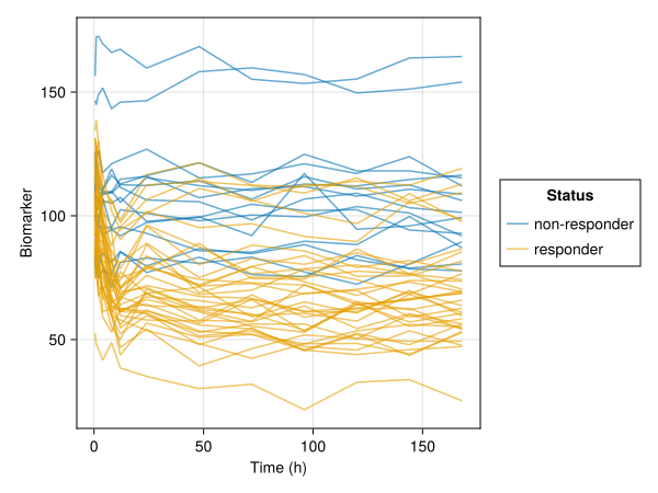
Here, the components are distinguished by their structure rather than by a component-specific parameter, so no special care is needed with the starting values beyond the usual:
init_pd = (;
    tvka = 1.5,
    tvcl = 4.0,
    tvvc = 25.0,
    tvr0 = 90.0,
    tvkout = 0.2,
    tvimax = 0.5,
    tvic50 = 2.0,
    Ω = Diagonal([0.1, 0.1, 0.1]),
    σ_pk = 0.2,
    σ_pd = 8.0,
    mixprobs = [0.5, 0.5],
)

fit_pd = fit(mix_pd, pop_pd, init_pd, FOCE(); optim_options = (; show_trace = false))
FittedPumasMixtureModel
Mixture model components: 2
Number of subjects: 50
Observation records: Active Missing
conc: 650 0
resp: 650 0
Total: 1300 0
Number of parameters: Constant Optimized
0 13
Likelihood approximation: FOCE
Likelihood optimizer: BFGS
Termination Reason: GradientNorm
Log-likelihood value: -1631.9049
-----------------------
Estimate
-----------------------
tvka 1.053
tvcl 3.3144
tvvc 29.868
tvr0 103.32
tvkout 0.097555
Ω₁,₁ 0.10805
Ω₂,₂ 0.097355
Ω₃,₃ 0.036378
σ_pk 0.15095
σ_pd 4.7238
tvimax 0.85066
tvic50 1.0853
mixprobs₁ 0.3
mixprobs₂ 0.7
-----------------------The classification recovers the responder status of every subject:
mean(subpopulation(fit_pd) .== true_subpopulation_pd)1.0With a week of daily biomarker measurements, a non-responder is easy to tell from a responder. The responsibility of the assigned component is close to one for every subject:
w_pd = responsibilities(fit_pd)
extrema(maximum, w_pd)
(0.9999106808898245, 1.0)Consequently, the penalty for the classification uncertainty is small and the ICL is close to the BIC:
(; bic = bic(fit_pd), icl = icl(fit_pd))(bic = 3357.0212911568997, icl = 3357.021471380141)The predictions and the empirical Bayes estimates of the inspection are computed per component, so a subject has a prediction under both the non-responder and the responder component:
predict(fit_pd)[end](SubjectPrediction(id = 50, ...), SubjectPrediction(id = 50, ...))inspect works as in the first example:
inspect_pd = inspect(fit_pd)
df_pd = DataFrame(inspect_pd)
[ Info: Calculating predictions.
[ Info: Calculating weighted residuals.
[ Info: Calculating empirical bayes.
[ Info: Evaluating dose control parameters.
[ Info: Evaluating individual parameters.
[ Info: Done.Plotting the individual predictions of both components against the observations of a subject shows what the mixture weighs for each subject. The predictions can be evaluated on a fine time grid with the obstimes keyword, and the DataFrame of the predictions has one row per subject, time point and component. For subject 3, a non-responder, the responder component predicts a suppression of the biomarker that is absent from the data. For subject 40, a responder, the non-responder component can only place a flat line through the observations, and the first day of the treatment is clearly not flat. The responsibilities, taken from the inspection, reflect this:
df_subjects = @chain df_pd begin
    @select :id :probability₂
    unique
    @rtransform :panel = "Subject $(:id), P(responder) = $(round(:probability₂; digits = 3))"
end
df_pred = @chain DataFrame(predict(fit_pd; obstimes = 0:0.5:168)) begin
    @rsubset :id in ("3", "40")
    @rtransform :component = labels_pd[:mixture_component]
    innerjoin(df_subjects; on = :id)
end
df_obs = @chain df_pop_pd begin
    @rsubset :id in ("3", "40")
    innerjoin(df_subjects; on = :id)
end

plt_pred =
    data(df_pred) *
    mapping(
        :time => "Time (h)",
        :resp_ipred => "Biomarker";
        color = :component => sorter(labels_pd) => "Component",
        layout = :panel,
    ) *
    visual(Lines) +
    data(df_obs) *
    mapping(:time => "Time (h)", :resp => "Biomarker"; layout = :panel) *
    visual(Scatter; color = :black)
draw(plt_pred; facet = (; linkyaxes = :none), figure = (; size = (900, 400)))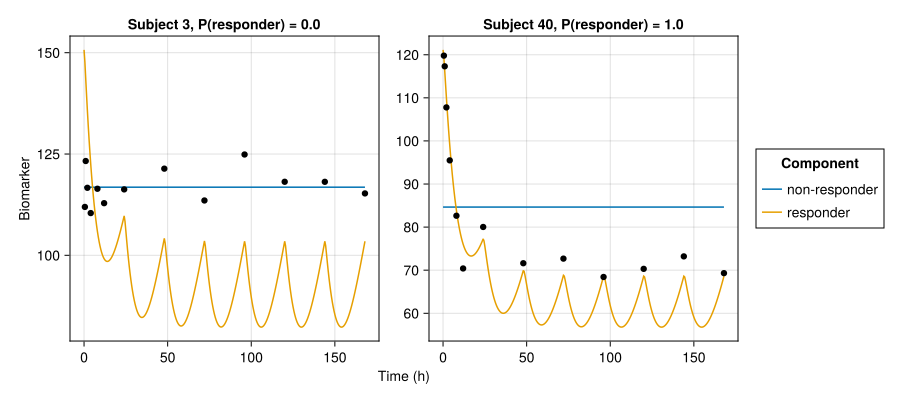
Limitations
The following are not supported for PumasMixtureModel in this release. Except for the first item, which fails with a MethodError, they are rejected with an informative error:
- The components must be defined with
@model.@emmodelcomponents and theSAEMestimation method are not supported. MAPestimation and the Bayesian methodsBayesMCMC,MarginalMCMCandJointMAP. ADirichletmixture probability parameter can be declared, but its prior is not used by the maximum likelihood fit.- The
MCEMestimation method inPumas.Experimental. vpc. The marginal NPDE and EWRES diagnostics cover the simulation based goodness-of-fit assessment of a mixture.
The DataFrame of a mixture inspection only contains the columns of the first component. Individual parameters and dynamic variables that exist only in later components, like Imax and IC50 of the responder component above, are therefore missing from the table.
Docstrings
Pumas.Experimental.PumasMixtureModel — Type
PumasMixtureModel(models::Tuple{Vararg{PumasModel}}, mixprobs::Pair{Symbol, <:Union{SimplexDomain, Dirichlet}})A mixture of PumasModels. The marginal likelihood for a subject is
$L(y|\theta) = \sum_k \pi_k L_k(y|\theta_k)$
where $\pi_k$ are the mixture probabilities (estimated as part of the parameter vector) and $\theta_k$ is the subset of parameters needed by submodel $k$.
Parameters are shared by name: if two submodels both reference tvcl, the same value is used for both. The combined parameter set is the union of all submodel parameters plus a user-specified mixture probability parameter constrained to the unit simplex.
Constructor
PumasMixtureModel(models, :name => SimplexDomain(N))
PumasMixtureModel(models, :name => Dirichlet(N, 1.0))
Constructs a mixture model from a tuple of PumasModels and a mixture probability specification. The specification is a Pair mapping a parameter name to either a SimplexDomain (flat prior) or a Dirichlet distribution (informative prior). The number of probabilities must match the number of models. All submodels that define a parameter with the same name must declare it identically, whether as a domain or as a prior distribution.
Random effects and diagnostics such as predict, empirical_bayes, wresiduals, icoef and dosecontrol are per-component quantities: they are given and returned as a Tuple with one entry per submodel, in the order the submodels were passed to the constructor. For a population the result is a Vector of such tuples, one per subject.
Pumas.Experimental.responsibilities — Function
responsibilities(fpm::FittedPumasMixtureModel) -> Vector{Vector{Float64}}Per-subject posterior component probabilities (responsibilities, a.k.a. IPmix): for subject i and component k,
wᵢₖ = πₖ exp(-nllᵢₖ) / Σⱼ πⱼ exp(-nllᵢⱼ),where πₖ are the (population) mixture probabilities and nllᵢₖ is subject i's marginal negative log-likelihood under component k. Returns one probability vector (summing to 1) per subject. See also subpopulation.
Pumas.Experimental.subpopulation — Function
subpopulation(fpm::FittedPumasMixtureModel) -> Vector{Int}Most-probable component (MAP / NONMEM MIXEST) for each subject, i.e. argmaxₖ wᵢₖ of the responsibilities.
Pumas.Experimental.icl — Function
icl(fpm::FittedPumasMixtureModel) -> Float64Integrated Completed Likelihood for choosing the number of mixture components. Uses the completed-data form ICL = -2·ℓc + dof·log(nobs), where the completed log-likelihood ℓc = Σᵢ log(π_ẑᵢ · Lᵢ,ẑᵢ) evaluates each subject under its most-probable component ẑᵢ = argmaxₖ wᵢₖ (subpopulation). Equivalently ICL = BIC - 2·Σᵢ log(maxₖ wᵢₖ), i.e. BIC plus a penalty for classification uncertainty. Lower is better; unlike BIC it favors mixtures whose components are well separated.
Introduced by Biernacki, Celeux & Govaert (2000); see McLachlan & Peel (2000), Finite Mixture Models, for the finite-mixture/classification framing.
Pumas.SimplexDomain — Type
SimplexDomain(n::Int)Specifies a parameter as a probability vector of length n constrained to the unit simplex (all elements non-negative, summing to 1). The initial value is a uniform distribution fill(1/n, n).