Custom Correlation Models
The Getting started example uses the built-in AffineTimeLinearModel, which maps dissolution to absorption through affine time-scaling and a linear fraction map. This guide demonstrates how to define a custom AbstractCorrelationModel by implementing the correlation interface — useful when the dissolution–absorption relationship is non-linear or requires domain-specific parameterization.
Simulated data
first(pk_df, 8)| Row | id | formulation | time | conc |
|---|---|---|---|---|
| Int64 | String | Float64 | Float64 | |
| 1 | 1 | FormA | 0.0 | 0.0 |
| 2 | 1 | FormA | 0.479017 | 0.252104 |
| 3 | 1 | FormA | 0.940682 | 0.766301 |
| 4 | 1 | FormA | 1.5166 | 1.48553 |
| 5 | 1 | FormA | 2.0618 | 2.15264 |
| 6 | 1 | FormA | 2.50108 | 2.64725 |
| 7 | 1 | FormA | 3.05358 | 3.17229 |
| 8 | 1 | FormA | 3.45924 | 3.49077 |
Defining a custom correlation model
To use the flexible interface, define a subtype of AbstractCorrelationModel whose fields are the model parameters (with a no-argument constructor), and implement four methods:
default_parameter_specs— defaultParameterSpeclist; names must match the struct's fields, in field ordercorrelation_vivo_to_vitro_time— map in vivo time to in vitro timecorrelation_vitro_to_vivo_time— the inverse time mapcorrelation_dissolution_to_absorption— map fraction dissolved to fraction absorbed
A model whose parameters include a time (a shift or a lag) also declares them through time_parameters, so the fit converts them between the data's time unit and magnitudes and scales their restarts to the observed time span.
This example replicates the built-in affine model to demonstrate the interface:
struct DemoAffineModel <: AbstractCorrelationModel
    abs_scale::Float64
    abs_intercept::Float64
    time_scale::Float64
    time_shift::Float64
end
DemoAffineModel() = DemoAffineModel(1.0, 0.0, 1.0, 0.0)

InVitroInVivoCorrelation.default_parameter_specs(::DemoAffineModel) = [
    ParameterSpec(:abs_scale, 1.0),
    ParameterSpec(:abs_intercept, 0.0),
    ParameterSpec(:time_scale, 1.0, 1e-6, 100.0),
    ParameterSpec(:time_shift, 0.0),
]
InVitroInVivoCorrelation.time_parameters(::DemoAffineModel) = [:time_shift]

function InVitroInVivoCorrelation.correlation_vivo_to_vitro_time(m::DemoAffineModel, t_vivo)
    t = Float64.(collect(t_vivo))
    return m.time_scale .* t .+ m.time_shift
end

function InVitroInVivoCorrelation.correlation_vitro_to_vivo_time(m::DemoAffineModel, t_vitro)
    t = Float64.(collect(t_vitro))
    return (t .- m.time_shift) ./ m.time_scale
end

function InVitroInVivoCorrelation.correlation_dissolution_to_absorption(m::DemoAffineModel, frac_diss)
    f = Float64.(collect(frac_diss))
    return m.abs_scale .* f .+ m.abs_intercept
end

correlation_model = DemoAffineModel()
parameter_specs = default_parameter_specs(correlation_model)
4-element Vector{InVitroInVivoCorrelation.ParameterSpec{Float64}}:
ParameterSpec(:abs_scale, 1.0, -Inf, Inf)
ParameterSpec(:abs_intercept, 0.0, -Inf, Inf)
ParameterSpec(:time_scale, 1.0, 1.0e-6, 100.0)
ParameterSpec(:time_shift, 0.0, -Inf, Inf)Running the pipeline
Pass the correlation_model and parameter_specs to run_ivivc:
result = run_ivivc(
    pk_df,
    diss_df;
    fast_formulation = "IV",
    validation_formulation = "FormB",
    times = collect(range(0.0, 48.0, length = 101)),
    correlation_model = correlation_model,
    parameter_specs = parameter_specs,
);
Model parameters
coeftable(result.model)| Row | parameter | constant | estimate |
|---|---|---|---|
| Symbol | Bool | Float64 | |
| 1 | abs_scale | false | 0.9896 |
| 2 | abs_intercept | false | 0.00185422 |
| 3 | time_scale | false | 0.841655 |
| 4 | time_shift | false | -0.0835769 |
Plots
concentration_profiles(result)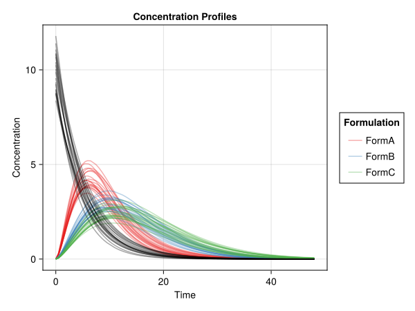
dissolution_profiles(result)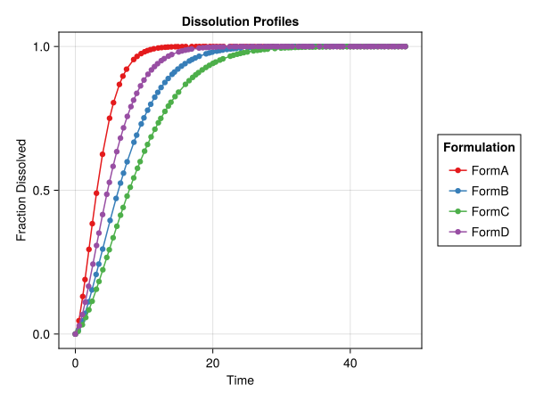
absorption_profiles(result)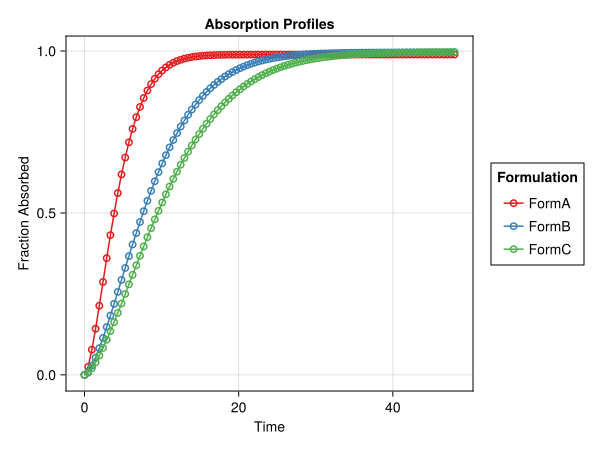
levy_plot(result)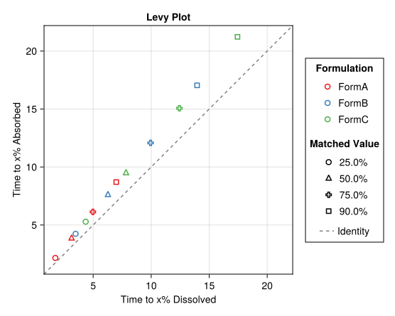
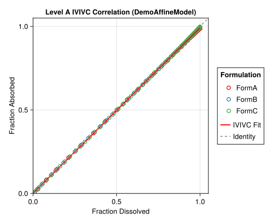
ivivc_correlation(result)