Noisy & Sparse Data
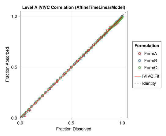
The Getting started example uses dense, noise-free simulated data. This guide applies realistic measurement noise (5% proportional CV + additive component) and sparse clinical sampling (15 PK timepoints) to verify that the IVIVC pipeline degrades gracefully under conditions typical of bioanalytical LC-MS/MS assays.
Key design choices that mirror real practice:
- Sparse PK sampling: 15 timepoints (dense around absorption, sparse in the terminal phase)
- Dissolution every 1 h: 49 timepoints (standard for automated dissolution baths)
- IV data stays clean: numerical deconvolution is sensitive to IV noise with sparse data
- Dissolution stays clean: matching real IVIVC workflows where dissolution is measured precisely in vitro
Simulated data
first(pk_df, 8)8×4 DataFrame
| Row | id | formulation | time | conc |
|---|---|---|---|---|
| Int64 | String | Float64 | Float64 | |
| 1 | 1 | FormA | 0.0 | 0.00888018 |
| 2 | 1 | FormA | 0.5 | 0.261667 |
| 3 | 1 | FormA | 1.0 | 0.871849 |
| 4 | 1 | FormA | 2.0 | 1.99015 |
| 5 | 1 | FormA | 4.0 | 3.82135 |
| 6 | 1 | FormA | 6.0 | 4.17208 |
| 7 | 1 | FormA | 8.0 | 3.60427 |
| 8 | 1 | FormA | 12.0 | 1.88451 |
first(diss_df, 8)8×3 DataFrame
| Row | formulation | time | diss |
|---|---|---|---|
| String | Float64 | Float64 | |
| 1 | FormA | 0.0 | 0.0 |
| 2 | FormA | 1.0 | 0.117503 |
| 3 | FormA | 2.0 | 0.297811 |
| 4 | FormA | 3.0 | 0.477703 |
| 5 | FormA | 4.0 | 0.632121 |
| 6 | FormA | 5.0 | 0.752796 |
| 7 | FormA | 6.0 | 0.840724 |
| 8 | FormA | 7.0 | 0.901237 |
Running the pipeline
The run_ivivc call is identical to the Getting started example — the pipeline handles noisy, sparse data without any special flags.
result = run_ivivc(
    pk_df,
    diss_df;
    fast_formulation = "IV",
    validation_formulation = "FormB",
    times = collect(range(0.0, 48.0, length = 101)),
);
Model parameters
coeftable(result.model)4×3 DataFrame
| Row | parameter | constant | estimate |
|---|---|---|---|
| Symbol | Bool | Float64 | |
| 1 | abs_scale | false | 0.993701 |
| 2 | abs_intercept | false | -0.00097586 |
| 3 | time_scale | false | 0.82112 |
| 4 | time_shift | false | -0.0110936 |
Plots
concentration_profiles(result)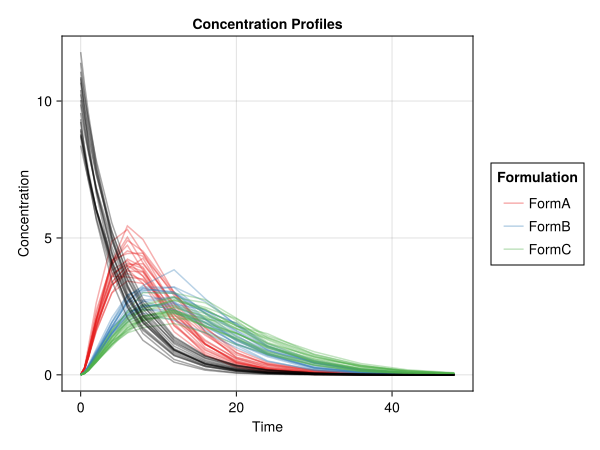
dissolution_profiles(result)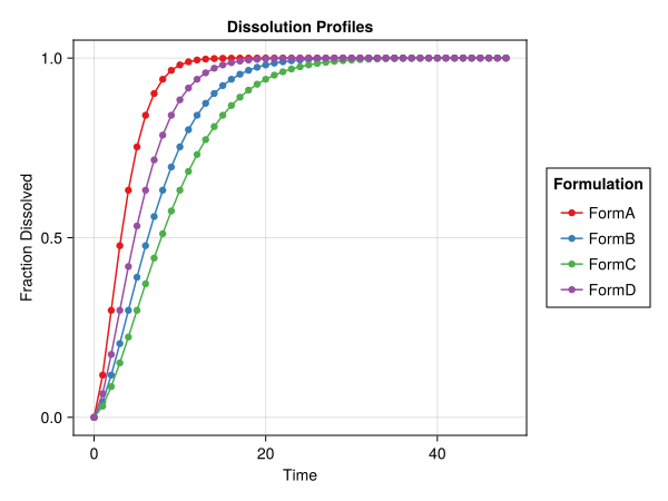
absorption_profiles(result)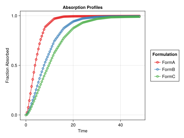
levy_plot(result)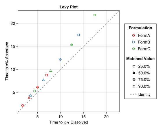
ivivc_correlation(result)