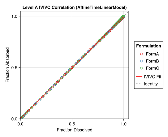
The Getting started example uses an IV bolus as the reference formulation for UIR fitting. This guide shows how to use an immediate-release (IR) oral formulation instead, using strip_ka=true to mathematically separate first-order absorption from the underlying disposition — useful when IV data is unavailable.
The data is identical to the Getting started example except that the reference formulation is an IR oral product with first-order absorption (rate constant $K_a$) and a lag time, rather than an IV bolus. Twenty subjects in a crossover design receive the IR reference and three oral test formulations.
first(pk_df, 8)
| Row | id | formulation | time | conc |
|---|
| Int64 | String | Float64 | Float64 |
|---|
| 1 | 1 | FormA | 0.0 | 0.0 |
| 2 | 1 | FormA | 0.479017 | 0.252104 |
| 3 | 1 | FormA | 0.940682 | 0.766301 |
| 4 | 1 | FormA | 1.5166 | 1.48553 |
| 5 | 1 | FormA | 2.0618 | 2.15264 |
| 6 | 1 | FormA | 2.50108 | 2.64725 |
| 7 | 1 | FormA | 3.05358 | 3.17229 |
| 8 | 1 | FormA | 3.45924 | 3.49077 |
first(diss_df, 8)
| Row | formulation | time | diss |
|---|
| String | Float64 | Float64 |
|---|
| 1 | FormA | 0.0 | 0.0 |
| 2 | FormA | 0.521124 | 0.0463696 |
| 3 | FormA | 1.07457 | 0.130579 |
| 4 | FormA | 1.41023 | 0.189439 |
| 5 | FormA | 1.9815 | 0.294384 |
| 6 | FormA | 2.46701 | 0.383808 |
| 7 | FormA | 3.07383 | 0.489692 |
| 8 | FormA | 3.95187 | 0.625072 |
The key difference from the Getting started example: strip_ka=true tells the pipeline that the reference formulation ("IR") is an oral formulation whose first-order absorption must be mathematically stripped to recover the underlying disposition. time_lag=true adds a lag-time parameter, and n_exp=1 sets the number of disposition exponentials.
result = run_ivivc(
    pk_df,
    diss_df;
    fast_formulation = "IR",
    strip_ka = true,
    time_lag = true,
    n_exp = 1,
    validation_formulation = "FormB",
    times = collect(range(0.0, 48.0, length = 101)),
);
first(result.uir_df, 8)
| Row | id | formulation | uir |
|---|
| Any | String | PolyExpo… |
|---|
| 1 | 3 | IR | PolyExponential{Float64, Float64}([8.65163], [0.209544], 1.0, 1.0) |
| 2 | 2 | IR | PolyExponential{Float64, Float64}([9.56063], [0.167306], 1.0, 1.0) |
| 3 | 4 | IR | PolyExponential{Float64, Float64}([8.75111], [0.189256], 1.0, 1.0) |
| 4 | 5 | IR | PolyExponential{Float64, Float64}([9.86454], [0.187739], 1.0, 1.0) |
| 5 | 6 | IR | PolyExponential{Float64, Float64}([9.30618], [0.250098], 1.0, 1.0) |
| 6 | 13 | IR | PolyExponential{Float64, Float64}([11.343], [0.209333], 1.0, 1.0) |
| 7 | 8 | IR | PolyExponential{Float64, Float64}([10.778], [0.180712], 1.0, 1.0) |
| 8 | 7 | IR | PolyExponential{Float64, Float64}([11.0441], [0.172853], 1.0, 1.0) |
coeftable(result.model)
| Row | parameter | constant | estimate |
|---|
| Symbol | Bool | Float64 |
|---|
| 1 | abs_scale | false | 0.993381 |
| 2 | abs_intercept | false | 0.0017848 |
| 3 | time_scale | false | 0.84159 |
| 4 | time_shift | false | -0.0822501 |
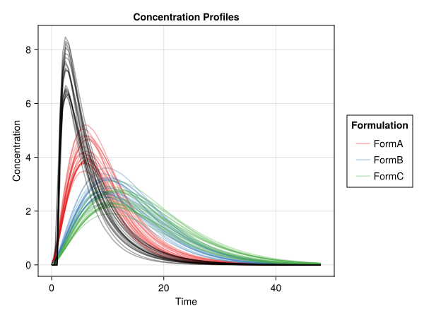
concentration_profiles(result)
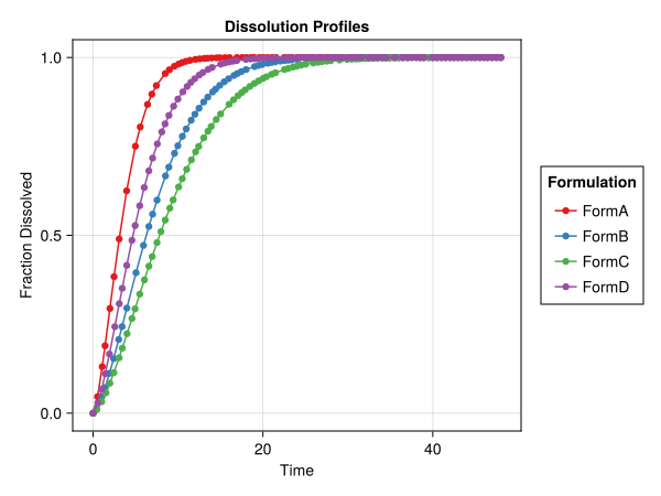
dissolution_profiles(result)
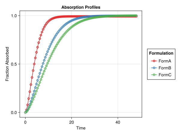
absorption_profiles(result)
levy_plot(result)
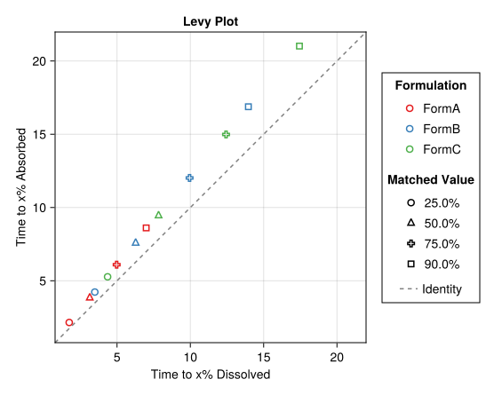
ivivc_correlation(result)