Parametric Dissolution Models
The Getting started example interpolates the dissolution data linearly. Dissolution can instead be smoothed with a parametric model fitted to each formulation's data: the fit irons out assay noise, evaluates cleanly between and beyond the sampled times, and summarises every profile in a few interpretable numbers. fit_dissolution does this and returns a DissolutionFit that goes into the pipeline in place of the raw data.
Models
Four standard sigmoidal forms are available. In all of them τ = max(t − tlag, 0), and the intercept int and lag tlag are held constant at zero unless you choose to estimate them.
| Model | Curve | Fitted by default |
|---|---|---|
HillDissolution | int + (finf − int) · τᵇ / (mdtᵇ + τᵇ) | finf, mdt, b |
WeibullDissolution | int + (finf − int) · (1 − exp(−(τ / mdt)ᵇ)) | finf, mdt, b |
DoubleWeibullDissolution | frac1-weighted sum of two Weibull terms | finf, frac1, mdt1, b1, mdt2, b2 |
MakoidBanakarDissolution | int + (fmax − int) · (τ / tmax)ᵇ · exp(b (1 − τ / tmax)) up to tmax, then fmax | fmax, tmax, b |
Simulated data
first(diss_df, 8)| Row | formulation | time | diss |
|---|---|---|---|
| String | Float64 | Float64 | |
| 1 | FormA | 0.0 | 0.0 |
| 2 | FormA | 0.521124 | 0.0463696 |
| 3 | FormA | 1.07457 | 0.130579 |
| 4 | FormA | 1.41023 | 0.189439 |
| 5 | FormA | 1.9815 | 0.294384 |
| 6 | FormA | 2.46701 | 0.383808 |
| 7 | FormA | 3.07383 | 0.489692 |
| 8 | FormA | 3.95187 | 0.625072 |
Fitting
Pass the dissolution data and a model form tag. Each formulation is fitted by least squares; the result shows the fitted parameters with the residual sum of squares and convergence per formulation:
diss_fit = fit_dissolution(diss_df, WeibullDissolution())DissolutionFit{WeibullDissolution}: 4 formulations, constant int, tlag
Row │ formulation finf mdt b int tlag rss converged
─────┼───────────────────────────────────────────────────────────────────────────
1 │ FormA 1.00001 4.00173 1.49831 0.0 0.0 7.80794e-7 true
2 │ FormB 1.00001 8.00064 1.49945 0.0 0.0 1.26759e-6 true
3 │ FormC 1.00001 10.0007 1.49977 0.0 0.0 6.70013e-7 true
4 │ FormD 1.00001 6.0011 1.49935 0.0 0.0 7.7115e-7 trueThe Simulated Data is generated from a Weibull with shape 1.5 and scales 4, 8, 10 and 6 h for FormA–FormD that dissolves completely, so the fit recovers mdt ≈ 4, 8, 10, 6, b ≈ 1.5 and finf ≈ 1 (the data are resampled linearly from the exact curve, hence the third decimal). int and tlag are held constant at zero unless asked otherwise. The parameters come back as a table, or per formulation as a named tuple or as the callable model:
coeftable(diss_fit)| Row | formulation | finf | mdt | b | int | tlag |
|---|---|---|---|---|---|---|
| String | Float64 | Float64 | Float64 | Float64 | Float64 | |
| 1 | FormA | 1.00001 | 4.00173 | 1.49831 | 0.0 | 0.0 |
| 2 | FormB | 1.00001 | 8.00064 | 1.49945 | 0.0 | 0.0 |
| 3 | FormC | 1.00001 | 10.0007 | 1.49977 | 0.0 | 0.0 |
| 4 | FormD | 1.00001 | 6.0011 | 1.49935 | 0.0 | 0.0 |
coef(diss_fit, "FormA")(finf = 1.000011690591569, mdt = 4.001726175000524, b = 1.4983079707420182, int = 0.0, tlag = 0.0)weibull_a = dissolution_model(diss_fit, "FormA")
weibull_a([1.0, 4.0, 12.0])3-element Vector{Float64}:
0.11769205554770891
0.6318901317475902
0.9944013225036943Constant and starting values
constantcoef names the parameters held constant at their initial value, and param sets that value. The tuple is the full set, so pinning the plateau at complete dissolution keeps the two default constants in the list. Without param, finf would be held at its default start, the observed maximum, which is not 1 for a profile that has not finished:
pinned = fit_dissolution(
    diss_df, WeibullDissolution();
    constantcoef = (:finf, :int, :tlag), param = (; finf = 1.0),
)
coeftable(pinned)| Row | formulation | finf | mdt | b | int | tlag |
|---|---|---|---|---|---|---|
| String | Float64 | Float64 | Float64 | Float64 | Float64 | |
| 1 | FormA | 1.0 | 4.00164 | 1.49835 | 0.0 | 0.0 |
| 2 | FormB | 1.0 | 8.0005 | 1.49949 | 0.0 | 0.0 |
| 3 | FormC | 1.0 | 10.0006 | 1.4998 | 0.0 | 0.0 |
| 4 | FormD | 1.0 | 6.001 | 1.49938 | 0.0 | 0.0 |
Dropping tlag from constantcoef estimates a lag time, here started at half an hour (the simulated profiles have none):
coeftable(fit_dissolution(diss_df, WeibullDissolution(); constantcoef = (:int,), param = (; tlag = 0.5)))| Row | formulation | finf | mdt | b | int | tlag |
|---|---|---|---|---|---|---|
| String | Float64 | Float64 | Float64 | Float64 | Float64 | |
| 1 | FormA | 1.00001 | 4.00173 | 1.49831 | 0.0 | 1.0367e-9 |
| 2 | FormB | 1.00001 | 8.00064 | 1.49945 | 0.0 | 1.04288e-9 |
| 3 | FormC | 1.00001 | 10.0007 | 1.49977 | 0.0 | 1.05718e-9 |
| 4 | FormD | 1.00001 | 6.0011 | 1.49935 | 0.0 | 1.0524e-9 |
Bounds live with the model and starting values are read off each profile; default_parameter_specs shows what a profile starts from:
form_a = diss_df[diss_df.formulation .== "FormA", :]
default_parameter_specs(WeibullDissolution(), form_a.time, form_a.diss)
5-element Vector{InVitroInVivoCorrelation.ParameterSpec{Float64}}:
ParameterSpec(:finf, 1.0, 0.0, 1.5)
ParameterSpec(:mdt, 4.009609922731674, 0.0, Inf)
ParameterSpec(:b, 1.0, 0.1, 10.0)
ParameterSpec(:int, 0.0, 0.0, 1.0)
ParameterSpec(:tlag, 0.0, 0.0, Inf)parameter_specs overrides these by name, so changing one bound is one ParameterSpec; everything else, including the default constants, stays:
coeftable(fit_dissolution(diss_df, WeibullDissolution(); parameter_specs = [ParameterSpec(:finf, 1.0, 0.0, 1.2)]))| Row | formulation | finf | mdt | b | int | tlag |
|---|---|---|---|---|---|---|
| String | Float64 | Float64 | Float64 | Float64 | Float64 | |
| 1 | FormA | 1.00001 | 4.00173 | 1.49831 | 0.0 | 0.0 |
| 2 | FormB | 1.00001 | 8.00064 | 1.49945 | 0.0 | 0.0 |
| 3 | FormC | 1.00001 | 10.0007 | 1.49977 | 0.0 | 0.0 |
| 4 | FormD | 1.00001 | 6.0011 | 1.49935 | 0.0 | 0.0 |
Comparing model forms
rss gives the residual sum of squares per formulation. The Hill curve cannot match the Weibull-generated data, and the numbers say so:
hill_fit = fit_dissolution(diss_df, HillDissolution())
DataFrame(formulation = diss_fit.formulations, Weibull = rss(diss_fit), Hill = rss(hill_fit))| Row | formulation | Weibull | Hill |
|---|---|---|---|
| String | Float64 | Float64 | |
| 1 | FormA | 7.80794e-7 | 0.017949 |
| 2 | FormB | 1.26759e-6 | 0.0256613 |
| 3 | FormC | 6.70013e-7 | 0.0244105 |
| 4 | FormD | 7.7115e-7 | 0.0242597 |
Running the pipeline
The fit takes the place of the dissolution DataFrame:
result = run_ivivc(
    pk_df,
    diss_fit;
    fast_formulation = "IV",
    validation_formulation = "FormB",
    times = collect(range(0.0, 48.0, length = 101)),
);
Model parameters
coeftable(result.model)| Row | parameter | constant | estimate |
|---|---|---|---|
| Symbol | Bool | Float64 | |
| 1 | abs_scale | false | 0.988818 |
| 2 | abs_intercept | false | 0.00264283 |
| 3 | time_scale | false | 0.84087 |
| 4 | time_shift | false | -0.0878416 |
result.pe_summary_df| Row | formulation | auc_predicted | auc_observed | pe_auc | cmax_predicted | cmax_observed | pe_cmax |
|---|---|---|---|---|---|---|---|
| String | Float64 | Float64 | Float64 | Float64 | Float64 | Float64 | |
| 1 | FormB | 49.9867 | 50.456 | 0.930165 | 2.85171 | 2.87857 | 0.933208 |
Plots
result.dissolution_df holds the fitted curves evaluated on the data's time grid, so the dissolution plot shows the smoothed profiles:
dissolution_profiles(result)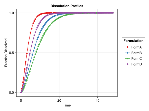
concentration_profiles(result)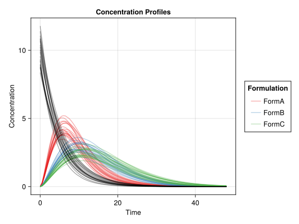
absorption_profiles(result)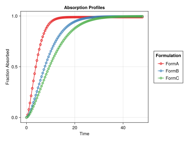
levy_plot(result)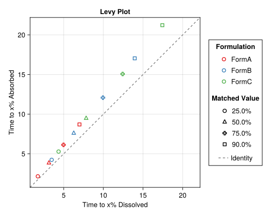
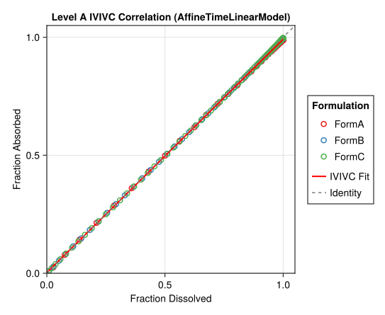
ivivc_correlation(result)